Ancient World: Tracing History With Genetic Dating

Every human being carries a living chronicle of the past. Embedded in the sequence of four chemical bases—adenine, thymine, cytosine, and guanine—that make up our DNA is a record of every migration, every encounter, every mixture that brought our ancestors from the first hominins of Africa to the diverse populations of the present day.

But this record is not written in plain language. It is encrypted in the patterns of genetic variation, in the lengths of ancestral DNA segments, in the frequencies of mutations shared across continents. The science of genetic dating provides the key to decrypting this record.

Genetic dating is the set of methods that use DNA to assign times to evolutionary events: the divergence of species, the migration of populations, the admixture of previously separated groups, and the expansion of lineages.

Unlike archaeological dating (radiocarbon, dendrochronology) which measures the age of artifacts, genetic dating reads the clock that ticks inside every living cell; the mutation rate.

This paper is a comprehensive guide to the principles, methods, and applications of genetic dating. It is written for the curious reader who wants to move beyond headlines like “Neanderthals interbred with humans 50,000 years ago” and understand how scientists actually arrive at such numbers.

We will begin with the deepest past and work our way forward to the admixture events that shaped modern South Asians, Europeans, and others. Along the way, we will explore:

• The molecular clock and why it is both powerful and controversial.

• Divergence dating: how we estimate when two species or populations last shared a common ancestor.

• Admixture dating: how we calculate how many generations have passed since two populations mixed, using the decay of ancestral DNA segments.

• The tools of the trade: PCA, qpAdm, DATES, ROLLOFF, and more.

• The pitfalls and controversies: mutation rate calibration, contamination, small sample sizes, and the interpretation of results.

• Extended case studies: from the Yamnaya expansions to the formation of Ancestral North and South Indians.

By the end, you will not only understand what genetic dates mean but also how to critically evaluate them; separating robust conclusions from speculative estimates. And you will appreciate the profound truth that genetic dating reveals: that human history is not a tree of pure branches but a tangled web of mixture, movement, and memory.

Part I: The Molecular Clock – Time’s Ticker in the Genome

Let's start with mutation. Think of your DNA as a very long sentence written with only four letters: A, T, C, G. Every time a cell divides to make new cells, it copies this sentence. But copying is not perfect. Occasionally, a mistake happens: an A becomes a G, or a T becomes a C. These mistakes are called mutations.

Most mutations are harmless; like a typo in a recipe that doesn’t change the taste of the cake. Some are harmful, and a very few are helpful. But here’s the key: mutations happen at a fairly steady rate, like a clock ticking.

The Clock Analogy

Imagine two identical books sitting on a shelf. Every year, a few random typos appear in each book. After 100 years, the two books will have many different typos. If you compare them and count the differences, you can estimate how long they have been apart.

Now replace “books” with “populations.” If two groups of humans separate (say, one stays in Africa and one moves to Europe), their DNA will start accumulating different mutations. The more differences you find, the longer they have been separated.

That is the molecular clock. By counting mutations and knowing the tick rate (how often mutations happen per year), you can calculate the time since two populations split.

How Do Scientists Know the Tick Rate?

This is a challenge. You cannot just guess how often mutations happen. Scientists have to calibrate the clock using events whose age is already known from other evidence (like fossils or archaeology).

For example, the oldest known human‑chimpanzee fossil is about 7 million years old. Scientists compare human and chimp DNA, count the differences, and then divide by 7 million years to get a mutation rate. Once you have that rate, you can use it to date other splits.

However, different calibration methods give different rates. A rate based on counting mutations in families (parents vs. children) is about twice as fast as a rate based on ancient fossils. This means genetic dates can vary by a factor of two depending on which rate you choose. Always check which rate a study used.

Divergence Dating in Action: Humans vs. Neanderthals

Neanderthals were our closest extinct relatives. When scientists sequenced the Neanderthal genome, they compared it to modern human genomes and counted the differences. Using a fossil‑calibrated rate, they calculated that the human and Neanderthal lineages split about 550,000 to 750,000 years ago.

That does not mean they never met again. In fact, they interbred later, around 50,000‑60,000 years ago. But the split date tells us when the two lineages became separate evolutionary paths.

Key takeaway: Divergence dating answers “when did two populations last share a common ancestor?” Admixture dating (next section) answers “when did two previously separated populations mix?”

---

Read Now

---

Part II: Admixture Dating – When Populations Mix

Divergence dating works for populations that split apart. But human history is full of mixing; when two groups that had been separate for thousands of years came together and had children.

How do you date such a mixing event? You cannot use mutation counts, because the mixed population inherits mutations from both sides. Instead, you use a different clock: the breaking up of DNA segments.

The DNA Quilt Analogy

Imagine you have two quilts: one red and one blue. You cut both quilts into small squares, then sew them together to make a new, mixed quilt. The first generation has large patches of red and large patches of blue.

Now suppose every generation, you take the quilt, cut each square into smaller pieces, and randomly resew them. With each generation, the red and blue patches become smaller and more scrambled. After many generations, the quilt looks uniformly pink (mixed), and the individual patches are tiny.

The rule: The average size of the original red or blue patches tells you how many generations have passed since the quilts were first mixed. Longer patches = more recent mixing. Shorter patches = older mixing.

Translating the Analogy to DNA

Your DNA comes in pieces called chromosomes. You inherit one copy of each chromosome from your mother and one from your father. When your body makes eggs or sperm, it shuffles the chromosomes, cutting and recombining them. This process is called recombination.

If your ancestors came from two different populations (say, Population A and Population B), your DNA will contain chunks of A‑ancestry and chunks of B‑ancestry. The boundaries between chunks are places where recombination happened in a past generation. Over time, recombination breaks the chunks into smaller and smaller pieces.

Therefore, if we measure the average length of A‑ancestry chunks in your genome, we can calculate how many generations ago your ancestors mixed.

The Math (Made Simple)

The relationship is surprisingly simple:

Average chunk length (in a unit called centiMorgans or cM) = 100/number of generations since admixture

Or, rearranged:

Generations since admixture = 100/average chunk length (cM)

Example: If the average chunk of Steppe ancestry in a population is 2 cM, then:

Generations = 100/2 = 50 generations

If we assume 25 years per generation, that is 50 × 25 = 1,250 years ago.

Different Methods for Measuring Chunks

Scientists have developed several computer programs to measure these ancestry chunks and calculate dates:

• ROLLOFF | 2012 | Measures how quickly DNA chunks decay | Modern DNA, large samples

• DATES | 2020 | Improved version that works with ancient DNA | Ancient skeletons, smaller samples

• GLOBETROTTER | 2014 | Can detect multiple mixing events | Complex histories (three or more sources)

A Real Example: Steppe Ancestry in South Asia

Scientists wanted to know when the Steppe pastoralists (ancestors of the Yamnaya and Andronovo cultures) mixed with the local population of South Asia.

They took DNA from modern South Asians and measured the average chunk length of Steppe ancestry. The average chunk was about 2.5 cM. Using the formula:

Generations = 100/2.5 = 40 generations

At 28 years per generation, that gives 40 × 28 = 1,120 years ago (around 800 AD). But that date is far too recent; it would mean Steppe people arrived in India in medieval times, contradicting all archaeology.

What went wrong? The problem is that after the initial mixing, South Asian populations kept mixing with each other, which further broke down the chunks. The chunk length in modern people reflects not just the original mixing but also thousands of years of internal mixing.

The solution: Scientists used ancient DNA from the Swat valley in Pakistan dated to 1200‑800 BC. Those ancient people had chunks that were still long. They compared the chunk lengths between the ancient Swat people and modern South Asians, and calculated that the original mixing happened around 1500‑1000 BC. That matches the archaeological timeline of the Gandhara Grave culture.

The calculation isn't a single, simple formula, but a two-step process of measuring and then projecting backwards in time. Let's break down the logic and then look at the specific numbers from the key study.

The Logic: How We Get from a Skeleton to a Date

Think of it like measuring a sound to figure out when it was made:

The Sample: You have an ancient skeleton from the Swat Valley dated to, say, 1200 BC by archaeological methods (like radiocarbon dating).

The Measurement (Admixture Dating): You analyze the DNA of this person and measure the average length of "Steppe ancestry" chunks in their genome. The DATES program does this. The key principle is that longer chunks mean more recent admixture, because there hasn't been as much time for them to be broken down.

The Projection (The Calculation): The measurement tells you the admixture happened a certain number of generations before the person lived. Let's say the average chunk length was 4 cM (centiMorgans). The relationship is roughly Generations = 100 / Average Chunk Length (cM).

So, 100 / 4 cM = 25 generations before the person lived.

If we assume a generation is 28 years (a common estimate used in these studies), then 25 generations × 28 years/generation = 700 years before the person lived.

If the person lived in 1200 BC, then 1200 BC + 700 years = 1900 BC. That's the calculated date for the admixture event.

The Specific Numbers from the Narasimhan et al. 2019 Study

This exact logic was applied in the landmark paper on South Asian genetics. While the detailed supplementary materials are technical, the key results are clear:

The study estimated the admixture event between the Steppe pastoralists and the local population of the Swat Valley occurred approximately 50-80 generations before the individuals studied lived.

Using a standard generation length of 28 years (which is common in the field for ancient populations), this timeframe translates to an admixture event that happened roughly 1,400 to 2,240 years before the skeletons were buried.

The skeletons were dated to around 1200-800 BC. Therefore, the mixing event itself is calculated to have taken place between approximately 1900 BC and 1500 BC.

Putting It All Together: The Numbers in the Formula

So, the calculation uses these key numbers:

Average Chunk Length: The DATES program measures this directly from the DNA, and for the Swat Valley individuals, it produced a value that, when plugged into the formula, indicated ~25-40 generations of decay.

Generations Since Admixture: This was calculated to be approximately 25 to 40 generations before the individuals lived.

Generation Length: The researchers assumed 28 years per generation for this population.

Archaeological Age: The Swat Valley skeletons are dated to c. 1200-800 BC.

The final output—the date of the mixing event—is a range of 1900-1500 BC. This matches the 1900-1500 BC range we saw.

This provides the specific numbers and the logical steps that connect the raw genetic data (the length of DNA chunks) to the calculated historical date (when the mixing happened).

What this means? Admixture dating works best when you have ancient DNA as a “time anchor.”

Part III: Haplogroups – Tracing Single Lines of Ancestry

Your DNA is a mix from all your ancestors. But two special parts of your DNA are passed down unchanged from a single parent:

• Y‑chromosome: Passed from father to son. Only males have it.

• Mitochondrial DNA (mtDNA): Passed from mother to all her children (both sons and daughters).

Because these do not recombine (they are not shuffled), they form lineages that can be traced back thousands of years.

A haplogroup is a branch on the family tree of Y‑chromosomes or mtDNA. Each haplogroup is defined by specific mutations that happened once in history and were then passed down.

Analogy: Think of a family surname. A haplogroup is like a genetic surname. Everyone in haplogroup R1a shares a common male ancestor who lived thousands of years ago.

How Haplogroups Are Used for Dating

By counting the mutations that have accumulated on a haplogroup branch, and knowing the mutation rate, scientists can calculate the TMRCA (Time to Most Recent Common Ancestor) of all people in that haplogroup.

Example: Haplogroup R1a‑Z93 is common in South Asia and among ancient Sintashta (Steppe) males. Its TMRCA is about 5,500‑6,000 years ago. That means the common ancestor of all living R1a‑Z93 men lived around 4000‑3500 BC. This matches the time when the Steppe pastoralist culture was forming.

It's important to remember that haplogroup TMRCA is not the date of a migration. It is the date of a single ancestor. The migration that spread that haplogroup could have happened much later, when his descendants had grown into a large population.

The Y‑Chromosome Adam and Mitochondrial Eve

Every man alive today inherited his Y‑chromosome from a single man who lived in Africa. He is called Y‑chromosome Adam. He was not the only man alive at his time, but his Y‑lineage is the only one that survived.

Using genetic dating, scientists estimate that Y‑Adam lived between 120,000 and 300,000 years ago. Similarly, Mitochondrial Eve (the common ancestor of all living humans through the mother line) lived between 150,000 and 250,000 years ago.

Notice that the dates are ranges, not single numbers. That is because of the mutation rate controversy and because different studies use different methods.

Fun fact: Adam and Eve of Africa (not Adam and Eve from scripture) did not live at the same time. They lived tens of thousands of years apart, and they never met.

Limitations of Haplogroup Dating:

• Lineage loss: A haplogroup can disappear by chance (genetic drift). This does not mean the people died out; just that their particular Y‑lineage was not passed down.

• Single line: Haplogroups ignore most of your ancestry. You have thousands of ancestors, but only one Y‑line and one mtDNA line. Autosomal DNA (the rest of your genome) gives a much broader picture.

• Not a migration date: A haplogroup can be present in a population long before it spreads.

Rule of thumb: Use haplogroups to track deep ancestry, but use autosomal admixture dating for recent (last 10,000 years) migration events.

Haplogroups do not give only the oldest (deepest) ancestor. They give a nested hierarchy of ancestors, from the very ancient to the relatively recent.

Think of a haplogroup like a family surname that mutates over time.

The "root" haplogroup (e.g., Y‑chromosome haplogroup A) is the oldest; the common ancestor of all men. Branches (subclades) formed when new mutations occurred.

For example, haplogroup R1a is a subclade of R1, which is a subclade of R, which is a subclade of F, and so on.

Each subclade has its own Time to Most Recent Common Ancestor (TMRCA). That TMRCA is the age of that specific branch, not the age of the entire tree.

How Young a Haplogroup Can Be (Haplogroup | TMRCA (approx.) | What it tells us):

• Y‑chromosome A (root) | ~200,000 years ago | Deepest human Y lineage

• Y‑chromosome R1a | ~20,000‑25,000 years ago | Originated in Eurasia after the Out‑of‑Africa migration

• Y‑chromosome R1a‑Z93 | ~5,500‑6,000 years ago | Specific branch that spread with Steppe pastoralists into South Asia

• Mitochondrial haplogroup M | ~60,000 years ago | Originated in South Asia after the coastal migration

• Mitochondrial haplogroup M2 | ~40,000‑50,000 years ago | A younger branch found in India

As you go down the tree to more specific subclades, the TMRCA becomes younger; sometimes just a few thousand years old.

So What Do Haplogroups Give? They give both ancient and recent information. The key is the level of resolution. A coarse haplogroup (like just "R1a") tells you about an ancient expansion.

A fine‑grained subclade (like "R1a‑Z93" or even more specific "R1a‑Y3") can tell you about migrations that happened within the last 2,000‑3,000 years.

Real‑World Example: Tracking the Steppe Migration

The root haplogroup R is very old (~30,000 years ago). It tells you nothing specific about the Steppe people.

R1a‑Z93 (a subclade) has a TMRCA of ~5,500 years ago. That matches the Sintashta/Andronovo culture.

An even younger subclade, R1a‑Z94, has a TMRCA of ~4,500 years ago and is found in South Asia. It may represent the actual founding lineage of the Indo‑Āryans.

Conclusion: Haplogroups are like a family tree. The trunk is old; the twigs are young. To answer recent historical questions, you look at the twigs, not the trunk.

Part IV: Visualizing Relationships – PCA Made Simple

Principal Component Analysis (PCA) is a way to take complex genetic data and turn it into a simple picture. It is like taking a 3D object and flattening it into a 2D shadow; you lose some detail, but you can still see the shape.

A PCA plot has two axes (PC1 and PC2). Each dot represents one individual (or one population average). Dots that are close together are genetically similar. Dots that are far apart are genetically different.

Reading a PCA Plot: The Steppe Example

Imagine a PCA of ancient and modern Europeans:

• Early farmers (LBK culture): Plot in one region.

• Western Hunter‑Gatherers (WHG): Plot in another region.

• Yamnaya (Steppe herders): Plot in a third region, between the farmers and the hunter‑gatherers.

• Corded Ware (Bronze Age Europeans): Plot exactly in the middle of a triangle connecting Yamnaya, farmers, and hunter‑gatherers.

What does this tell us? Corded Ware people were a mix of all three ancient populations. The PCA shows this visually: they are “pulled” toward each source.

Using PCA for Dating

PCA does not give dates directly. But it helps you decide which populations should be dated. If an ancient population falls between two modern populations, that is a clue that admixture happened. You then use admixture dating (DATES, ROLLOFF) to find out when.

Part V: How Scientists Actually Do Genetic Dating

Let us walk through a real study to see all the pieces come together.

The Big Question (What we want to know): We have a population of ancient people who lived in the Swat Valley of Pakistan around 1200 BC. We want to know: were they a mixture of two older groups, the BMAC people (from Central Asia) and the Steppe herders (from the Eurasian grasslands)? If yes, in what proportions (e.g., 70% BMAC + 30% Steppe)? And when did that mixing happen?

Step 0: What we start with — Nothing but dirt and bones

Scientists go to archaeological sites in Swat Valley. They dig up skeletons from graves. Each skeleton is carefully cleaned, dated using radiocarbon (carbon dating), and given a label: Swat_1200BC, Swat_800BC, Swat_300BC. They also collect blood or saliva from living South Asians (Rors, Pathans, Tamils, etc.) for comparison.

At this point, we only have physical bones and tubes of saliva. No DNA yet.

Step 1: From bones to computer files — Sequencing DNA

What happens: In a special clean lab, scientists grind a small piece of bone into powder. They use chemicals to extract the DNA. This DNA is broken into tiny fragments (ancient DNA degrades).

They put these fragments into a sequencing machine that reads the order of the letters (A, T, C, G) in each fragment. The machine outputs a huge computer file; a list of millions of short DNA sequences.

Example of raw output: `AGCTTAGCTA...` (but a million lines of that).

The problem: These fragments are jumbled. They need to be assembled like a jigsaw puzzle. To do that, they need a reference picture.

The reference genome: Imagine a complete, correct map of a human genome; all 3 billion letters in order. This map was created years ago by sequencing several people and stitching them together. It's like a master dictionary. Scientists align each fragment from the skeleton against this reference map. The computer figures out where each fragment belongs.

Result after this step: For the Swat_1200BC skeleton, we now have a file that contains a list of positions on the genome (e.g., position 1,000,001) and what letter is present at that position (A, T, C, or G). But because the DNA is degraded, we only get one letter per position (pseudohaploid; we don't get both copies from mother and father). That's enough for the next steps.

Same process is done for BMAC skeletons, Steppe skeletons, and modern South Asians. Now we have computer files (genomes) for many individuals.

Step 2: Understanding what we have — The "genetic data"

At the end of Step 1, we have a table (very large) like this (Individual | Position 1,000,001 | Position 1,000,002 | ... ):

• Swat_1200BC | A | G | ...

• BMAC_individual1 | A | C | ...

• Steppe_individual1 | T | G | ...

• Modern_Ror | A | G | ...

Each row is a person. Each column is a specific location in the genome. The letter is the DNA base at that location.

This is the "real data" we will use for all calculations.

Step 3: Finding the mixture proportions — qpAdm (the smoothie analogy)

Now we have three sets of genomes:

• Target: Swat_1200BC (the mystery)

• Sources: BMAC and Steppe (the possible ingredients)

• Outgroups: Very distant populations (e.g., African Yoruba, East Asian Han); these act as neutral reference points.

Why can't we just compare Swat to BMAC and Steppe directly? Direct comparison would only tell us: "Swat is more similar to BMAC than to Steppe." It would not tell us if Swat is a mixture of both, and it certainly would not tell us the exact percentages.

We need to create test mixtures. Imagine we mix 50% BMAC + 50% Steppe mathematically. We calculate what the DNA of a hypothetical person would look like at every position if they had exactly 50% ancestry from each. Then we compare that hypothetical person's DNA to the real Swat DNA. If they don't match well, we try another ratio (60/40, 70/30, etc.) until we find the best match.

But how do we compare? We don't compare letter by letter (that would be too noisy). Instead, we use a statistical tool called f₄-statistics. Think of it as a summary score that measures how much two populations share recent ancestry.

Simplified explanation of f₄-statistics: Imagine you have four populations: A, B, C, D. An f₄ statistic asks: "Do A and B share more genetic variants with each other than with C and D?" If the answer is zero, then A and B are equally related to C and D; they form a simple tree. If the answer is not zero, it indicates that A and B have mixed ancestry.

qpAdm uses many f₄-statistics to test whether the target can be expressed as a weighted average of the source populations. It tries different weights (x% BMAC + y% Steppe) and calculates how well the predicted f₄-statistics match the actual f₄-statistics calculated from the real data.

The algorithm works like this:

1. Start with a guess: 50% BMAC + 50% Steppe.

2. Compute predicted f₄-statistics for that mix.

3. Compare to real f₄-statistics from Swat DNA. Compute the difference (residual).

4. Adjust the percentages slightly (e.g., 51% BMAC, 49% Steppe) and recompute.

5. Keep adjusting in the direction that reduces the residual.

6. Stop when the residual is as small as possible. That gives the best-fit percentages.

In our case, the best fit was 70% BMAC + 30% Steppe.

Now the p-value: The p-value tells us whether the residual (the remaining difference) is small enough to be explained by random chance, or whether it's so large that our model is wrong. A p-value > 0.05 means "good fit" – the model is plausible. A p-value < 0.05 means "reject the model" – we need a third source.

The study reported a p-value > 0.05, so the 70/30 model is accepted.

Result of Step 3: We now know that the Swat_1200BC people were a mixture of approximately 70% BMAC ancestry and 30% Steppe ancestry.

Step 4: Dating the mixture — DATES (the chunk decay method)

Now we know what was mixed, but not when the mixing happened. Did the mixing occur 100 years before they lived? 1,000 years? 5,000 years?

The principle: When two populations mix, their children have long DNA chunks from each parent. Over generations, these chunks get broken into smaller pieces by recombination (the shuffling that happens when eggs and sperm are made). So: longer chunks = more recent mixing; shorter chunks = older mixing.

The chunk length measurement: In the Swat_1200BC genomes, the scientists look at the DNA segments that come from Steppe ancestry. They measure how long these segments are, on average. The unit is centiMorgan (cM). Think of cM as a measure of length along a chromosome, where 1 cM roughly corresponds to 1 million DNA letters.

The formula: If the average Steppe chunk length is L cM, then the number of generations since mixing is approximately:

Generations} = 100/L

Why 100? Because 100 cM is roughly the length of a whole chromosome, and recombination breaks chunks at a rate of about 1 break per 100 cM per generation. It's a standard approximation.

Calculation for Swat_1200BC: The average Steppe chunk length was about 4 cM.

Generations = 100/4 = 25 generations

Now we need to convert generations to years. Scientists use an estimate of 28 years per generation for ancient populations (this accounts for age of reproduction).

Years since admixture = 25 * 28 = 700 years

So the mixing happened 700 years before the Swat_1200BC individuals lived.

When did those individuals live? Radiocarbon dating tells us they lived around 1200 BC. So the mixing event occurred at:

1200 BC + 700 years = 1900 BC

Result of Step 4: The admixture (mixing of BMAC and Steppe) happened around 1900 BC.

Step 5: Checking with later samples — Does the pattern hold?

If our date is correct, then in later Swat individuals (800 BC and 300 BC), the Steppe ancestry chunks should be shorter because more generations of recombination have passed.

For Swat_800BC:

• Average chunk length = 2 cM.

• Generations = 100 / 2 = 50 generations.

• Years = 50 × 28 = 1400 years before they lived.

• They lived at 800 BC, so admixture date = 800 + 1400 = 2200 BC? That would be older than 1900 BC – a problem.

Wait, this seems inconsistent. But careful: The 2 cM measurement is the average chunk length in the Swat_800BC individuals. That length includes the decay that happened between the original mixing (1900 BC) and the time they lived (800 BC). So the calculation should give the same original mixing date if we do it correctly.

Actually, the formula `Generations = 100 / L` gives the total number of generations from the mixing event to the person's lifetime. For Swat_800BC, if the mixing happened at 1900 BC, then the time difference is 1900 - 800 = 1100 years.

1100/28 ≈ 39

At 28 years/gen, that's about 39 generations. Then predicted average chunk length = 100 / 39 ≈ 2.56 cM. The measured 2 cM is close enough given sampling error and the fact that chunk lengths are not perfectly uniform.

So the data are consistent: the same original mixing event explains both the 1200 BC and 800 BC samples.

Result of Step 5: The dating is consistent across multiple time points, strengthening confidence.

Step 6: Compare with archaeology and linguistics

Archaeology: The Gandhara Grave culture appears in Swat around 1600-1200 BC. Its artifacts show a mix of local (BMAC-related) and Steppe features. That matches our genetic mixing date of 1900-1500 BC.

Linguistics: The Rigveda, composed around 1500-1200 BC, describes the Sarasvati river as a mighty, snow-fed river. Geological evidence shows that the Sarasvati dried up around 1900 BC. So the Rigveda must have been composed before that date. This aligns with the Steppe migration happening before 1900 BC.

Final answer: Steppe admixture in South Asia happened between 1900 and 1500 BC.

Summary Table (Step | What we do | Input | Output | What it tells us):

1. Collect | Excavate skeletons, get modern blood | Archaeological sites, volunteers | Physical samples | Which people we will study

2. Sequence | Extract DNA, read letters, align to reference | Bone powder, blood | Digital genomes (A,T,C,G files) | The raw genetic data

3. qpAdm | Test mixture proportions using f4-statistics | Target, sources, outgroups | 70% BMAC + 30% Steppe, p>0.05 | The ancestry composition

4. DATES | Measure Steppe chunk lengths, apply formula | Swat_1200BC genome | 1900 BC | When mixing happened

5. Consistency | Repeat for later samples | Swat_800BC, Swat_300BC | Same mixing date | Confirms the date

6. Archaeology/Linguistics | Compare with independent evidence | Gandhara grave culture, Rigveda | Agreement | Validates the story

Frequently asked questions:

Q: Why do we need both ancient and modern DNA?

A: Ancient DNA gives us direct snapshots of past populations. Modern DNA tells us how those ancient populations contributed to people alive today. But for dating admixture, ancient DNA is better because the chunks are longer and less decayed.

Q: What is a centiMorgan (cM)?

A: It's a unit of genetic distance. 1 cM means there is a 1% chance that a recombination event will occur between two points on a chromosome in one generation. It roughly corresponds to 1 million DNA letters. For chunk length, larger cM means physically longer DNA segment.

Q: Why 28 years per generation?

A: It's an average age of having children in ancient societies, considering that people had children over a span of years, not all at age 20. It's an approximation; using 25 or 30 would change the date by a few centuries, but not dramatically.

Q: How do we know which chunks are Steppe ancestry?

A: By comparing the Swat genome to a reference Steppe genome (from Sintashta or Andronovo skeletons). The computer identifies segments that match the Steppe pattern more closely than the BMAC pattern.

Q: Could the mixing have happened in multiple waves?

A: Yes, but the simple model assumes one pulse. If there were multiple pulses, the average chunk length would give a weighted average date. The consistency with archaeology suggests a single major pulse around 1900-1500 BC.

Part VI: How to Read DNA Analysis?

This guide will give you a practical framework for interpreting Y‑DNA (paternal) and mtDNA (maternal) haplogroups. It’s structured like a reference manual: first the rules, then examples from around the world, and finally a simple checklist to decode any haplogroup you encounter.

Part I: The Absolute Basics – What Are Haplogroups?

Your DNA contains two special sections that are passed down without being shuffled (recombined) each generation:

• Y‑DNA | only males | the direct paternal line | father → son only

• mtDNA (mitochondrial DNA) | everyone | the direct maternal line | mother → all her children

The Haplogroup Family Tree Analogy: Think of a haplogroup like a family surname that mutates over time. The root of the tree is the oldest common ancestor. Every time a new mutation occurs, a new “branch” (called a subclade) is created.

The ISOGG Y‑DNA Haplogroup Tree provides a regularly updated reference for this branching structure.

Example: R1a‑Z93 is a branch of R1a, which is a branch of R, which is a branch of the very ancient F – and so on back to the root (A). The naming convention uses the root letter followed by numbers or letters indicating the nested branches.

The #1 Rule: The Deeper You Go, The More You Learn

If you see someone say “Haplogroup R1a,” that is like saying “my surname is Khan.” It tells you very little – there are Khans everywhere. But if you say “R1a‑Z93,” that is like saying “my specific Khan lineage from a particular village in Kashmir” – now you have something you can trace.

The most detailed sub‑branch is called a terminal SNP (Single Nucleotide Polymorphism). The terminal SNP represents the last known mutation unique to that lineage.

Therefore, always try to find the most specific subclade. The root letter (like R or E) tells a story of deep time; tens of thousands of years ago. The terminal SNP (like R1a‑Z93) tells a story of recent history; sometimes only 3,000‑5,000 years ago.

Part II: How to Read a Y‑DNA Haplogroup (Step by Step)

Let us use the example: R1a‑Z93. When you see this, here is the step‑by‑step process to extract information.

Step 1: Identify the Root Letter – “R”

Haplogroup R is one of the major branches of the Y‑chromosome tree. It originated approximately 30,000 years ago in Central Asia or Southern Siberia.

It is very common in Europe, Central Asia, and South Asia. Men with haplogroup R are direct paternal descendants of the man who first carried that defining mutation ~30,000 years ago.

Step 2: Identify the Major Branch – “R1a”

R1a is a specific subclade of R. It is defined by a mutation that occurred approximately 20,000‑25,000 years ago.

R1a is now found at high frequencies in Eastern Europe (Slavic countries), Central Asia, and South Asia. It is strongly associated with the spread of Indo‑European languages.

Step 3: Identify the Specific Subclade – “Z93”

Z93 is a mutation that occurred within the R1a branch, approximately 5,000‑6,000 years ago. It is the Asian branch of R1a, found today primarily in Central Asia, South Asia, and parts of the Middle East.

Step 4: Translate the Code

• R = a man who lived ~30,000 years ago in Central Asia.

• R1a = a descendant of that man who lived ~20,000‑25,000 years ago.

• R1a‑Z93 = a specific lineage within R1a that lived ~5,500 years ago in the steppes of Central Asia.

This lineage is strongly associated with the Sintashta and Andronovo cultures; the Bronze Age pastoralists who spoke early Indo‑Iranian languages and who later migrated into South Asia.

Therefore, an ancient skeleton with R1a‑Z93 is likely a male whose paternal ancestors were Steppe pastoralists who moved into South Asia around 2000‑1500 BC and contributed to the gene pool of South Asia (Iran, India, Afghanistan, Pakistan).

Part III: A World Tour of Major Haplogroups

Now you can use the same decoding method for any haplogroup. Below is a reference table of major Y‑DNA haplogroups from different continents, followed by detailed examples.

Table 1: Y‑DNA Haplogroups at a Glance (Haplogroup | Typical Region(s) | Approximate Age | Historical Association)

• A | Africa (Khoisan, Ethiopia) | ~200,000 years | Deepest human Y‑lineage; “Y‑Chromosome Adam”

• B | Africa (Pygmies, Hadza) | ~100,000 years | Ancient African lineage

• E1b1a | Sub‑Saharan Africa | ~40,000 years | Bantu expansion (Niger‑Congo languages)

• E1b1b | North Africa, Horn of Africa | ~30,000 years | Afro‑Asiatic languages

• J | Middle East, Caucasus, Mediterranean | ~40,000 years | Neolithic farmers, spread of agriculture

• J2 | Anatolia, Greece, Italy, India | ~30,000 years | Ancient Greek, Roman, and Indus Valley populations

• Q | Siberia, Native Americas | ~25,000 years | First peopling of the Americas

• R | Eurasia | ~30,000 years | Very broad Eurasian lineage

• R1a | Eastern Europe, Central Asia, South Asia | ~20,000 years | Indo‑European (especially Balto‑Slavic and Indo‑Iranian)

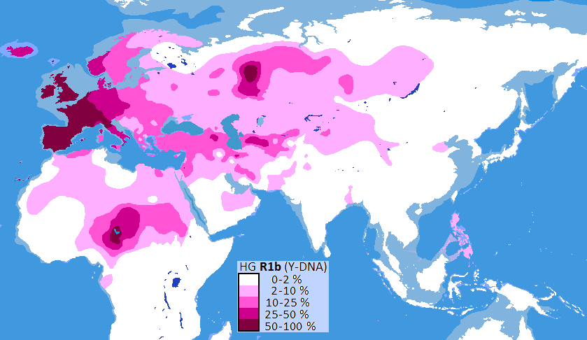
• R1b | Western Europe | ~20,000 years | Yamnaya, Celts, Bell Beaker culture

• O | East Asia, Southeast Asia | ~35,000 years | Han Chinese, Japanese, Korean, Vietnamese

• C | Siberia, Mongolia, Australia | ~50,000 years | Paleolithic Eurasian lineage

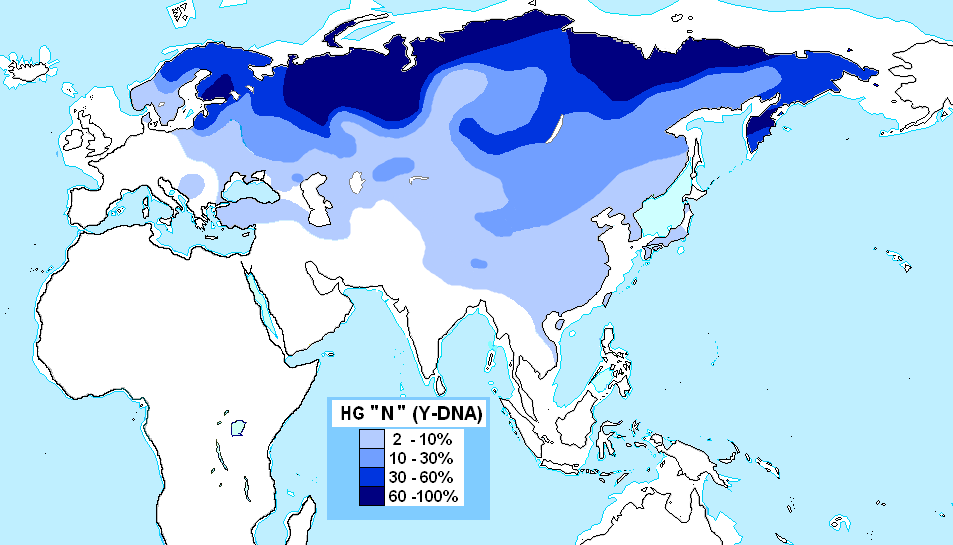
• N | Siberia, Northern Europe, Finland | ~20,000 years | Uralic language speakers

• H | South Asia (India) | ~30,000 years | Indigenous South Asian “AASI” lineage

• L | South Asia, Central Asia | ~30,000 years | Indus Valley and Central Asian populations

Case Study 1: Europe – R1b (The Yamnaya and Celtic Connection)

If you see R1b on a report:

• R = the root (ancient Central Asia).

• R1b = the western branch of R.

• R1b‑L21 = a specific subclade strongly linked to the Insular Celts of Ireland and Britain.

Historical interpretation: R1b originated ~20,000‑25,000 years ago. It was the dominant Y‑chromosome of the Yamnaya pastoralists who expanded into Europe around 3000‑2500 BC. In Britain, the arrival of R1b‑L21 around 2500 BCE is associated with the Bell Beaker culture, which replaced approximately 90% of the male population of the island within a few centuries.

Key point: R1b in Europe = Steppe ancestry (Yamnaya). R1b in Africa = more recent back‑migration or colonial era.

Case Study 2: East Asia – O (The Han Chinese Signature)

If you see O‑M122 (also called O2):

• O = the East Asian branch, originating ~35,000 years ago in Southeast Asia or southern China.

• O‑M122 = the subclade that dominates modern Han Chinese populations.

Historical interpretation: O‑M122 is found in 50‑60% of Han Chinese males and in 30‑40% of Korean and Vietnamese males. Its expansion is linked to the spread of Sino‑Tibetan languages and the Neolithic agricultural revolution in the Yellow and Yangtze River valleys.

Key point: O = East Asian origin. If you see O in Europe or the Middle East, it usually indicates recent migration (e.g., Silk Road traders, Mongol Empire).

Case Study 3: Africa – E1b1a (The Bantu Expansion)

If you see E1b1a (also called E‑M2):

• E = African branch.

• E1b1a = a subclade that originated in West or Central Africa ~40,000 years ago.

Historical interpretation: E1b1a is the dominant Y‑chromosome lineage among Bantu‑speaking peoples. Its rapid expansion over the past 3,000‑5,000 years tracks the spread of Bantu farmers from Cameroon/Nigeria across sub‑Saharan Africa. Today it is found from Senegal to South Africa and as far east as Kenya.

Key point: E1b1a in Africa = Niger‑Congo language family. E1b1a outside Africa = usually the colonial Atlantic slave trade of Europeans.

Case Study 4: The Americas – Q (The First Americans)

If you see Q‑M242:

• Q = the Siberian branch, originating ~25,000 years ago in Central Asia.

• Q‑M3 = a subclade that arose in Beringia or just after the first migration into the Americas.

Historical interpretation: Q is the pan‑American Y‑chromosome lineage. Approximately 90% of Native American males belong to haplogroup Q (the remainder are mostly C). The founding population of the Americas crossed the Bering land bridge from Siberia around 20,000‑25,000 years ago carrying Q and C lineages.

Key point: Q in the Americas = indigenous ancestry. Q in Europe or Asia = Siberian or Central Asian ancestry (e.g., Turkic peoples, Huns).

Case Study 5: South Asia – H (The Indigenous “AASI” Marker)

If you see H‑M69:

• H = a deep branch that originated in South Asia approximately 30,000‑40,000 years ago.

• H1a1 = a subclade associated with the Roma (Gypsy) migration out of India 1,500‑2,000 years ago.

Historical interpretation: Haplogroup H is often called the “Indian marker” because it is found at high frequencies in South India (25‑35%) and among tribal populations. It represents the paternal lineage of the Ancient Ancestral South Indian (AASI) hunter‑gatherers; the original inhabitants of the subcontinent before the arrival of Iranian farmers and Steppe pastoralists.

Key point: H in South India = deep indigenous ancestry. H in Europe = usually Roma heritage.

Part IV: The mtDNA (Maternal) Side

The same logic applies to mtDNA haplogroups, except they track the mother line.

• L | Africa | ~150,000 years | “Mitochondrial Eve”; all non‑African lineages descend from L3

• M | East Asia, South Asia | ~60,000 years | Early coastal migration out of Africa

• N | Eurasia | ~60,000 years | Sister branch of M; spread across Europe and Asia |

• R | Eurasia | ~50,000 years | Ancestral to many European and Asian lineages

• U | Europe, West Asia | ~50,000 years | Ancient European hunter‑gatherers; U5 is especially old

• H | Europe | ~25,000 years | Most common mtDNA in Europe today (~40%)

• J | Middle East, Europe | ~45,000 years | Neolithic farmers

• T | Europe, Middle East | ~30,000 years | Ancient European and Near Eastern populations

• A, C, D | Siberia, Americas | ~30,000 years | Native American founding lineages

Reading an mtDNA Example: U5a1

• U = a branch of macro‑haplogroup R, originating ~50,000 years ago in Western Asia.

• U5 = a subclade that arose ~35,000 years ago in Europe.

• U5a1 = a specific branch found among ancient Scandinavian hunter‑gatherers and modern Sami people.

Therefore, an ancient skeleton with U5a1 was likely a female whose maternal ancestors were among the earliest post‑Ice Age hunter‑gatherers of Northern Europe.

Part V: Practical Decoding – A Step‑by‑Step Checklist

When you see a haplogroup in a news article or a DNA report, ask these questions in order:

Step 1: Is it Y‑DNA or mtDNA?

If the letter is alone (e.g., “H”), check the context. For mtDNA, H is European. For Y‑DNA, H is Indian. If it has a lowercase “a” or “b” (e.g., U5a1), it is mtDNA. If it has numbers after a dash (e.g., R1a‑Z93), it is Y‑DNA.

Step 2: What is the root letter?

• A, B, E = Africa.

• C, N = Siberia / Northern Asia.

• O = East Asia.

• Q = Native America / Siberia.

• R = Europe / Central Asia / South Asia.

• H (Y‑DNA) = South Asia.

• L (mtDNA) = Africa (but L as Y‑DNA is different).

Step 3: How specific is the subclade?

• “R1a” is ancient and broad (~20,000 years).

• “R1a‑Z93” is recent and specific (~5,500 years).

• A terminal SNP (e.g., R1a‑Z93‑Y3) is the most precise.

Step 4: What does the distribution tell you?

• Use a database like YFull or ISOGG to look up where that subclade is found today.

• High frequency in a specific region = origin point.

• Low frequency in a distant region = migration or admixture.

Step 5: What is the archaeological association?

• R1b‑Z2103 = Yamnaya culture.

• R1a‑Z93 = Sintashta / Andronovo / Indo‑Iranian.

• O‑M122 = Han Chinese expansion.

• Q‑M3 = First Americans.

Part VI: Resources for Further Research

If you want to research a haplogroup on your own, use these free tools:

• YFull Y‑Tree | Interactive tree of all known Y‑DNA haplogroups; shows estimated ages and geographic distribution | yfull.com/tree

• ISOGG Y‑Tree | Regularly updated academic reference for Y‑DNA nomenclature | isogg.org/tree

• Wikipedia “Haplogroup X” | Each major haplogroup has a dedicated page with maps, history, and subclades | en.wikipedia.org

• FTDNA Haplotree | Commercial but large database of modern samples | familytreedna.com

• Mitomap | mtDNA reference database | mitomap.org

Part VII: The Golden Rules of Haplogroup Interpretation

One haplogroup does not define a person. It is a single line out of thousands. A man with R1a‑Z93 is 99%+ descended from other lineages. Haplogroups tell you where that single line came from, not the whole person.

Haplogroups are not races. An African man with R1b got it from a European or Near Eastern ancestor within the last 10,000 years. A European man with E1b1a got it from an African ancestor.

The deeper the subclade, the more recent the history. R1a tells you something about the Ice Age. R1a‑Z93 tells you something about the Bronze Age.

Always cross‑check with autosomal DNA. A skeleton with R1a‑Z93 but very low Steppe autosomal ancestry probably had a single Steppe male ancestor many generations ago.

Migrations are not necessarily invasions. Finding R1a in India does not automatically prove a violent 'Aryan invasion' of the kind described in 19th‑century colonial narratives.

However, the genetic and linguistic evidence is consistent with a small‑scale but sustained migration of Steppe pastoralist males—likely several thousand individuals over multiple generations—who established themselves as a dominant elite.

Their military and technological advantages (chariots, horse‑riding, bronze weapons) allowed them to spread their language and culture without requiring a massive population replacement or a single conquering army. This process, known as elite dominance, explains how a relatively small number of migrants could transform the linguistic and cultural landscape.

Summary: What You Can Say After Reading This Guide

When you see a post that says “Ancient skeleton from Swat Valley has R1a‑Z93,” you can now confidently say:

“That means this male’s direct paternal line traces back to a man who lived about 5,500 years ago on the Central Asian steppes, associated with the Sintashta or Andronovo cultures. His ancestors were Steppe pastoralists who moved southward and mixed with local BMAC and Indus Valley populations. This fits the archaeological picture of the Gandhara Grave culture and the linguistic spread of Indo‑Iranian languages into South Asia.”

You have just decoded the story hidden in a single line of code.

Let's explore the mixing. Let's say a Steppe pastoralist man (Y‑DNA = R) marries a Neolithic farmer woman (mtDNA = J). They have children.

Here is exactly what happens, step by step.

The parents

• Father | Steppe pastoralist (e.g., Yamnaya) | R (e.g., R1b or R1a) | (irrelevant for his children; men don't pass mtDNA) | 100% Steppe ancestry

• Mother | Neolithic farmer (e.g., Anatolian or European early farmer) | (women don't have Y) | J (a common mtDNA haplogroup of early farmers) | 100% Neolithic farmer ancestry

Their children

From the father:

• If the child is a son: The father's Y‑chromosome (R). Daughters get no Y.

• Half of the father's autosomal DNA (randomly shuffled); roughly 50% Steppe ancestry.

From the mother:

• All children (sons and daughters) get the mother's mtDNA (J).

• Half of the mother's autosomal DNA; roughly 50% Neolithic farmer ancestry.

What does this mean for haplogroups?

• The Y‑haplogroup R continues down the male line (sons of sons). It does not change into something else.

• The mtDNA haplogroup J continues down the female line (daughters pass it to all children, sons carry it but do not pass it).

• No new haplogroup is created. Haplogroups change only by rare mutations, not by mixing.

What happens if their descendants keep marrying into other groups?

Over generations, the Y‑R and mtDNA‑J will spread through the population, but they will remain separate markers. Meanwhile, the autosomal DNA will become a complex mosaic of Steppe, farmer, and possibly other ancestries.

Real‑world example: This exact scenario happened thousands of times during the Yamnaya expansion into Europe. Steppe males (R1b) married local Neolithic farmer women (who carried mtDNA haplogroups like H, J, T, K). Their children had R1b Y‑DNA and farmer mtDNA, and their autosomal DNA was mixed. That is why modern Europeans have Steppe Y‑chromosomes (R1b, R1a) but largely Neolithic farmer mtDNA.

---

Read Now

---

Part VII: Haplogroups Across the World

Before we dive into the specific branches of the human family tree, it's useful to understand how all these haplogroups fit together.

The diagram below shows the major branching points from Y‑chromosomal Adam down to the lineages that dominate different parts of the world today.

---

Africa (Haplogroups A & B)

These are the deepest branches of the human Y‑chromosome tree, representing the original inhabitants of Africa.

Haplogroup A – The earliest lineage, born around 275,000 years ago in northwestern or central Africa. It represents the deepest human Y‑lineage, and its carriers are almost exclusively found in Africa today. Subclades include A00 (found in a small population in Cameroon), A0, A1a, and A1b1.

---

Haplogroup B – A descendant of BT, originating around 100,000 years ago, also within Africa. It is commonly found among Pygmy peoples and hunter‑gatherer groups in West‑Central Africa. Its highest frequencies occur among the Baka (63‑72%), Hadzabe (52‑60%), and Nuer (50%) populations.

---

The Out of Africa Migration (Haplogroups C, DE, F)

These haplogroups represent the first modern humans to leave Africa and colonize the rest of the world.

Haplogroup CF – The ancestral lineage that split from the African lineage BT around 70,000 years ago, likely in Southwest Asia. All non‑African populations descend from CF.

Haplogroup DE – One of the two primary branches of CF, known for carrying the YAP+ (Y Alu Polymorphism) insertion, a unique genetic marker. It gave rise to two major branches: D and E.

---

Haplogroup F (F-M89) – The other primary branch of CF, originating around 55,000 years ago in South Asia/West Asia. This is the ancestor of most Eurasian haplogroups (G, H, I, J, K, L, M, N, O, P, Q, R). Over 90% of non‑African men belong to its descendant lineages.

---

Haplogroup C (C-M130) – Originating around 53,000 years ago in Southwest Asia, haplogroup C was among the earliest groups to leave Africa. It spread along the coasts of India and Southeast Asia to reach Australia and China.

Today, C is the predominant Y‑DNA lineage among many indigenous peoples of Central Asia, Siberia, East Asia, North America, and Australia. Its major subclade C2 (C-M217) is the most frequent branch, found mostly in Central Asia, Eastern Siberia, and significant frequencies in parts of East Asia.

---

Haplogroup D: The Jōmon and Tibetan Lineage

Haplogroup D (D-CTS3946) – Originating around 72,700 years ago, this lineage carries the YAP+ marker shared with E. It has two primary branches, D1 and D2, found primarily in East Asia, at low frequency in Central and Southeast Asia, and at very low frequency in Western Africa and Western Asia.

Haplogroup D is found in high frequencies among Japanese (25‑35%, the Jōmon lineage), Tibetans (50%+), and the Andaman Islands (90%+). The unique D1a2a subclade in Japan is one of the most distinctive Y‑DNA markers in the world, linking modern Japanese to the ancient Jōmon people who inhabited the archipelago over 15,000 years ago.

---

Haplogroup E: The African Backbone

Haplogroup E (E-M96) – The sibling of D within DE, E originated in Africa around 70,000 years ago and remains the most common Y‑DNA lineage across the continent. Its major subclades include:

• E1b1a (E-M2): The Bantu expansion lineage, dominant across sub‑Saharan Africa (70‑80% in Nigeria, Cameroon, and much of Central and Southern Africa). This lineage spread rapidly over the past 3,000‑5,000 years with the expansion of Bantu‑speaking farmers from West‑Central Africa.

• E1b1b (E-M215): Common in North Africa, the Horn of Africa, the Middle East, and Southern Europe. It is particularly associated with Berber, Egyptian, Somali, and Greek populations. Subclade E‑M81 is the Berber marker, while E‑V13 is common in the Balkans.

---

The Neolithic Farmer Lineages (Haplogroups G, H, I, J)

These haplogroups expanded with the spread of agriculture from the Fertile Crescent and other early farming centers.

Haplogroup G (G-M201) – Originating in the Middle East or South Asia around 30,000‑48,500 years ago, G is strongly associated with the spread of agriculture from Anatolia and the Caucasus into Europe. Its subclade G2a is found in Neolithic farmer skeletons across Europe.

Today, G is most common in the Caucasus, Iran, Anatolia, and Mediterranean Europe, with a global distribution across Europe, northern and western Asia, northern Africa, the Middle East, and South Asia.

---

Haplogroup H (H-M69) – Originating in South Asia (India) between 30,000 and 40,000 years ago, H is the primary Y‑DNA lineage of the Ancient Ancestral South Indians (AASI); the original hunter‑gatherer population of the subcontinent.

It is found at high frequencies among Dravidian‑speaking and tribal populations of India. The subclade H1a1a (H-M82) is also found among the Romani people, who originated in South Asia and migrated into the Middle East and Europe around the beginning of the 2nd millennium AD.

---

Haplogroup I (I-M170) – The only major Y‑DNA lineage that originated in Europe, I diverged from its parent IJ in Iran around 43,000 years ago. It is divided into two primary branches: I1 (Nordic), common in Scandinavia and Northern Europe, and I2 (Balkan), common in Southeast Europe and Sardinia.

I1 expanded rapidly during a migration from Scandinavia into Southern Sweden, Denmark, and Norway around 2000 BC. I2a was the main haplogroup found in Mesolithic Europe until the arrival of Anatolian farmers carrying G2a around 6000 BC.

---

Haplogroup J (J-M304) – Believed to have evolved in the Caucasus or Iran around 30,000‑42,900 years ago. It spread during the Neolithic, primarily into North Africa, the Horn of Africa, Europe, Anatolia, Central Asia, South Asia, and Southeast Asia.

Its two primary branches are J1 (J-M267), associated with Semitic‑speaking populations and common in the Arabian Peninsula, and J2 (J-M172), associated with the spread of agriculture from the Fertile Crescent and common in the Mediterranean, the Middle East, Iran, India, and the Caucasus.

---

The Great Eurasian Expansion (Haplogroup K)

Haplogroup K (K-M9) – An old lineage that arose approximately 47,000‑50,000 years ago, probably in South Asia/West Asia. Today, K and its descendant haplogroups are the patrilineal ancestors of most of the people living in the Northern Hemisphere, including most Europeans, Asians, and Native Americans. It gave rise to haplogroups L, M, N, O, P, Q, and R.

---

Haplogroup L (L-M20) – Associated primarily with South Asia and the Indus Valley Civilization, L is also found at lower frequencies in Central Asia, Southwest Asia, North Africa, and Southern Europe along the Mediterranean coast.

It is particularly common among the Baloch and Dravidian populations. Studies suggest a potential association between the migration of South Asian L1-M22 lineages and the spread of Dravidian languages.

---

Haplogroup M (M-P256) – Found predominantly in Melanesia, Micronesia, Polynesia, and eastern Indonesia. It is believed to have first appeared between 32,000 and 47,000 years ago.

---

Haplogroup N (N-M231) – Originated in East Asia, likely in northern China or Mongolia, around 15,000‑20,000 years ag. For about 6,500 years, N was almost exclusively the dominant paternal lineage in northeastern China before its carriers began migrating westward.

It spread counterclockwise across Siberia and into Northern Europe, where N1c is the majority Y‑chromosomal haplogroup among Finns (58%), Lithuanians (42%), Latvians (38%), and Estonians (34%). Haplogroup N is strongly associated with the spread of Uralic languages (Finnish, Estonian, Hungarian).

---

Haplogroup O (O-M175) – The dominant Y‑DNA lineage of East and Southeast Asia, O is believed to have first appeared in Siberia or eastern Central Asia approximately 35,000 years ago. It is the primary lineage of Han Chinese, Koreans, Japanese, Vietnamese, Thai, and other Austronesian populations.

Its major subclades are O1 (M119), found in Southeast Asia and Taiwan (linked to the Austronesian expansion), and O2 (M122), the most common subclade in East Asia, strongly associated with the spread of Sino‑Tibetan languages and the Neolithic agricultural revolution in the Yellow River valley.

---

Haplogroup P (P-P295) – The direct ancestor of both Q and R, P originated approximately 43,000 years ago, likely in South Asia. It spread from there to Central Asia and later into parts of Europe and the Americas.

Today, the haplogroup is found at low frequencies in India, Pakistan, and Central Asia, but its descendant lineages dominate most non‑African populations.

---

Haplogroup Q (Q-M242) – Originating in Central Asia around 25,000‑35,000 years ago, Q is the predominant Y‑DNA haplogroup among Native Americans, as well as several peoples of Central Asia and Siberia.

Its subclade Q-M3 occurred around 10,000‑15,000 years ago as the migration into the Americas was underway and is found in over 90% of indigenous peoples in Meso‑ and South America.

---

The Steppe Pastoralists (Haplogroup R)

Haplogroup R (R-M207) – A descendant of P, originating around 30,000‑35,000 years ago in Asian Steppe. It has three primary branches: R1a, R1b, and R2. The descendants of R are present throughout Europe, Central Asia, South Asia, and parts of West Asia, Africa, and North America.

Haplogroup R1a (R-M420) – Diverged from R1 around 15,000‑25,000 years ago. Its subclade M417 diversified around 3,400‑5,800 years ago. R1a is strongly associated with the spread of Steppe pastoralists (Yamnaya, Sintashta, Andronovo) and Indo‑European languages.

The Asian branch R1a‑Z93 is the primary lineage of Indo‑Iranian (Aryan) peoples, found at high frequencies in Central Asia, South Asia, and among Sintashta/Andronovo ancient DNA. The European branch R1a‑Z283 is common among Slavic and Baltic populations.

Haplogroup R1b (R-M343) – The most common Y‑DNA lineage in Western Europe, found at 70‑90% in Ireland, Scotland, Spain, and Portugal. Its subclade R‑L23 is the Yamnaya lineage, which spread into Europe from the Pontic‑Caspian steppe around 3000‑2500 BC. R‑U106 is common among Germanic populations, while R‑P312 is the Celtic/Italic branch.

Haplogroup R2 (R-M124) – Found primarily in South Asia, as well as in Central Asia, the Caucasus, the Middle East, and North Africa. It is particularly common among Sinhalese, Bengali, and Dravidian populations.

Summary: What Your Haplogroup Tells You

• A, B | Africa | Deepest human lineages; original hunter‑gatherers

• C | Central/East Asia, Oceania | Paleolithic coastal migration; Mongol, Australian Aboriginal, Native American

• D | East Asia (Japan, Tibet, Andamans) | Jōmon (Japan); Tibetan; Andamanese

• E | Africa, Mediterranean | Bantu expansion (E1b1a); Berber/Egyptian/Greek (E1b1b)

• F | Ancestral to most non‑Africans | Foundational Eurasian lineage

• G | Middle East, Caucasus, Europe | Neolithic farmers from Anatolia/Caucasus

• H | South Asia | AASI (Ancient Ancestral South Indians); Dravidian; Romani

• I | Europe | Indigenous European hunter‑gatherers; I1 (Nordic), I2 (Balkan)

• J | Middle East, Mediterranean, South Asia | Neolithic farmers; J1 (Semitic), J2 (Fertile Crescent agriculture)

• K | Ancestral to L, M, N, O, P, Q, R | Gateway to most Eurasian lineages

• L | South Asia, Central Asia | Indus Valley Civilization; Dravidian

• M | Melanesia, Polynesia | Pacific islanders; Papuan

• N | Siberia, Northern Europe | Uralic languages; Finnish, Estonian, Hungarian

• O | East, Southeast Asia | Han Chinese, Korean, Japanese, Austronesian

• P | Ancestral to Q and R | Siberian/Central Asian origin

• Q | Siberia, Americas | Native American founding lineage

• R | Eurasia, Americas | Ancestral to R1a, R1b, R2

• R1a | Eastern Europe, Central Asia, South Asia | Steppe pastoralists; Indo‑European (Slavic, Indo‑Iranian)

• R1b | Western Europe | Yamnaya; Celtic, Germanic, Italic

• R2 | South Asia, Central Asia | Sinhalese, Bengali, Dravidian

---

A Look mtDNA Haplogroups

Although both mtDNA and Y‑DNA are passed down uniparentally (mtDNA from mother to all children, Y‑DNA from father to sons), they trace different human histories because of fundamental differences in inheritance, mutation rate, and the social behavior of males versus females.

The Y‑chromosome mutates roughly twice as fast as mtDNA, so it accumulates more differences in the same time span, giving finer resolution for recent migrations. More importantly, migration has often been sex‑biased: conquests, trade, and elite dominance frequently involved long‑distance movement of males, while women tended to move shorter distances through marital exchange.

This is why, for example, the Y‑chromosome of a population can be almost completely replaced (as in Europe after the Yamnaya expansion) while the mtDNA remains largely local.

Out of Africa, both mtDNA haplogroups L3, M, and N left the continent, but their subsequent paths diverged because the earliest modern humans spread along coasts (favored by both sexes), while later expansions, such as the spread of agriculture or pastoralism, were often male‑driven.

Consequently, mtDNA haplogroups like H, J, and T reflect the movements of Neolithic farming women, whereas Y‑haplogroups like R1a and R1b track Bronze Age pastoralist men. Thus, comparing the two gives a fuller, sometimes contrasting, picture of human prehistory: mtDNA preserves deeper, more continuous maternal lineages, while Y‑DNA is more sensitive to recent male‑mediated demographic events.

Below is the mtDNA counterpart to the Y‑DNA guide we built. It follows the same structure: a reference of all major mtDNA haplogroups, followed by the same detailed format we used for Y‑DNA; one line per haplogroup with a short pointer on what it represents.

• L0 | ~150,000–200,000 | Southern Africa (or Southern East Africa) | Oldest human maternal lineage; associated with Khoisan peoples

• L1 | ~100,000–150,000 | Central/West Africa | Ancient African lineage; found in Pygmy groups

• L2 | ~70,000–100,000 | West Africa | Spread with Bantu expansion; common in sub‑Saharan Africa |

• L3 | ~60,000–80,000 | East Africa | The “Out of Africa” branch; ancestral to all non‑African haplogroups

• M | ~50,000–75,000 | South/Southeast Asia | One of two primary non‑African trunks; dominates East Asia, India, Oceania

• N | ~50,000–70,000 | Northeast Africa / West Asia | The other primary non‑African trunk; spread across Eurasia and the Americas

• R | ~50,000–70,000 | South Asia (or West Asia) | Major descendant of N; ancestral to most West Eurasian haplogroups

• HV | ~20,000–30,000 | West Asia / Europe | Ancestral to H and V

• H | ~20,000–25,000 | West Asia / Europe | Most common mtDNA in Europe (~40‑50%); post‑LGM expansion

• V | ~12,000–15,000 | Southwestern Europe (Iberian Peninsula) | Autochthonous European; post‑LGM expansion from Iberian refugium

• U | ~45,000–60,000 | West Asia / Europe | Oldest European maternal lineage; associated with hunter‑gatherers

• K | ~12,000–30,000 (subclade K1 ~22,000) | West Asia / Europe | Subclade of U8; found in Ötzi the Iceman

• J | ~40,000–45,000 | West Asia / Middle East | Neolithic farmer lineage; common in the Near East, Europe, North Africa

• T | ~25,000–30,000 | Middle East / Near East | Derived from JT; associated with Neolithic expansions

• X | ~30,000 | West Asia / Middle East | Unique; found in Europe, Near East, and among Native Americans (as a founder)

• I | ~20,000–30,000 | West Asia / Near East | Uncommon West Eurasian lineage; associated with post‑LGM expansions

• W | ~20,000–30,000 | West Asia / Near East | Uncommon West Eurasian lineage; associated with post‑LGM expansions

• A | ~30,000–60,000 | East Asia | Native American founder (A2); also common in Siberia and East Asia

• B | ~30,000–50,000 | East Asia | Native American founder (B2); prevalent along Asian coasts

• C | ~30,000–60,000 | East Asia / Siberia | Native American founder (C1); common in Siberia and Central Asia

• D | ~30,000–60,000 | East Asia / Siberia | Native American founder (D1); frequent in East Asia and Siberia

• E | ~8,000–11,000 | Coastal South China / Taiwan | Associated with Austronesian expansion

• F | ~20,000–45,000 | East / Southeast Asia | Common in southern China and Southeast Asia

• G | ~27,000–40,000 | Northeast Asia | Found in Northeast Asia and around the Sea of Okhotsk

• Z | ~20,000–30,000 | Northeast Asia / Siberia | Subclade of M; found in Saami, Finns, and Siberians

Africa

Haplogroup L0 – The oldest human maternal lineage, originating 150,000–200,000 years ago in Southern Africa or Southern East Africa. It is associated with the Khoisan peoples and represents the deepest branch of the human mtDNA tree.

Haplogroup L1 – Originated in Africa 100,000–150,000 years ago. Found in Central and West African populations, including Pygmy groups.

Haplogroup L2 – Originated in West Africa 70,000–100,000 years ago. Spread widely across sub‑Saharan Africa with the Bantu expansion.

Haplogroup L3 – Originated in East Africa 60,000–80,000 years ago. It is the ancestral branch from which all non‑African haplogroups (M, N, and R) descend, marking the “Out of Africa” migration.

The Out of Africa Expansion

Haplogroup M – One of the two primary non‑African trunks, originating 60,000–75,000 years ago in Asia. It is found across East Asia, Southeast Asia, India, Oceania, and the Americas. Its descendants include C, D, E, G, Q, and Z.

Haplogroup N – The other primary non‑African trunk, originating 50,000–70,000 years ago in Northeast Africa or West Asia. It spread across Eurasia and the Americas, giving rise to haplogroups A, B, F, I, W, X, and the major West Eurasian trunk R.

Haplogroup R – A major descendant of N, originating 50,000–70,000 years ago, likely in South Asia. It is ancestral to most West Eurasian mtDNA lineages, including HV, H, V, U, K, J, and T.

Europe & West Eurasia

Haplogroup HV – Ancestral to H and V, originating 20,000–30,000 years ago in West Asia or Europe. It represents a pre‑LGM lineage that diversified after the ice sheets retreated.

Haplogroup H – The most common mtDNA haplogroup in Europe, accounting for 40–50% of the population. It originated 20,000–25,000 years ago in West Asia or Europe and spread after the Last Glacial Maximum.

Haplogroup V – An autochthonous European haplogroup, originating 12,000–15,000 years ago in the Iberian Peninsula. It spread from a southwestern European refugium after the LGM and is found at elevated frequencies among the Saami of northern Scandinavia.

Haplogroup U – One of the oldest European maternal lineages, originating 45,000–60,000 years ago. It is associated with Paleolithic hunter‑gatherers and remains present in Europe today (~11% of the population). Its subclade U5 is particularly ancient.

Haplogroup K – A subclade of U8, originating 12,000–30,000 years ago in West Asia or Europe. It is found in Europe, North Africa, and South Asia. Ötzi the Iceman (c. 5300 years ago) belonged to subclade K1.

Haplogroup J – Originated 40,000–45,000 years ago in West Asia / Middle East. Associated with Neolithic farmers, it spread into Europe, North Africa, and South Asia. Subclade J2b is found in the Indus Valley and India.

Haplogroup T – Originated 25,000–30,000 years ago in the Near East. Derived from JT, it is associated with Neolithic expansions and is found across Europe, the Middle East, and North Africa.

Haplogroup X – Diverged from N about 30,000 years ago, likely in West Asia. It is found in Europe (~2% of the population), the Near East, North Africa, and – uniquely – as a founding lineage among Native Americans (X2a).

Haplogroup I – An uncommon West Eurasian lineage, originating in the Near East during the LGM or pre‑warming period.

Haplogroup W – Another uncommon West Eurasian lineage, also originating in the Near East during the LGM or pre‑warming period.

East Asia, Siberia & The Americas

Haplogroup A – Originated in East Asia 30,000–60,000 years ago. Its subclade A2 is one of the five founding maternal lineages of Native Americans. Found across Siberia and East Asia.

Haplogroup B – Originated in East Asia 30,000–50,000 years ago. Subclade B2 is a founding Native American lineage. Prevalent along the coasts of Asia and among Austronesian populations.

Haplogroup C – Originated in East Asia or Siberia 30,000–60,000 years ago. Subclade C1 is a founding Native American lineage. Common in Siberia, Central Asia, and East Asia.

Haplogroup D – Originated in East Asia or Siberia 30,000–60,000 years ago[reference:18]. Subclade D1 is a founding Native American lineage. Frequent in East Asia, Siberia, and the Americas.

Haplogroup E – A relatively young haplogroup, originating 8,000–11,000 years ago on the north Fujian coast (South China). Strongly associated with the Austronesian expansion: it traveled to Taiwan with Neolithic settlers ~6,000 years ago and spread across Maritime Southeast Asia with the Austronesian language dispersal.

Haplogroup F – Originated in East or Southeast Asia 20,000–45,000 years ago. Common in southern China and Southeast Asia. Descended from R9.

Haplogroup G – Originated in East or Northeast Asia 27,000–40,000 years ago[reference:21]. Found at highest frequencies in indigenous populations around the Sea of Okhotsk and in Northeast Siberia. Descended from M.

Haplogroup Z – Originated in Northeast Asia or Siberia 20,000–30,000 years ago. A subclade of M found among Saami, Finns, and Siberian populations.

Summary: What Your mtDNA Haplogroup Tells You

• L0, L1, L2, L3 | Africa | Deepest human lineages; “Mitochondrial Eve” (L)

• M, N, R | Asia (founding lineages) | Out of Africa trunks; ancestral to all non‑Africans

• H, V, U, K, J, T, X, I, W | Europe & West Asia | Post‑glacial expansions; Neolithic farmers; hunter‑gatherers

• A, B, C, D | East Asia, Siberia, Americas | Founding lineages of Native Americans (A2, B2, C1, D1)

• E | Southeast Asia / Taiwan | Austronesian expansion

• F | East / Southeast Asia | Southern China and Southeast Asia

• G, Z | Northeast Asia / Siberia | Indigenous Northeast Asian and Siberian populations

It also helps to understand why comparing Y‑DNA and mtDNA is so revealing. The two inheritance systems are like parallel chronicles: Y‑DNA records the history of fathers and sons, while mtDNA records mothers and all children.

Because they are inherited independently, any mismatch between them points directly to sex‑biased behavior in the past; differential migration, marriage patterns, warfare, or reproductive success.

When both tell the same story, migration likely involved whole families. When they diverge, we know something unusual happened: men moved without women, or women were absorbed from conquered groups, or social structures like patrilocality or polygyny skewed the genetic record.

The following observations are the most striking examples of such mismatches across the globe, each revealing a hidden chapter in human history.

1. The European Neolithic: Farmer Women, Hunter‑Gatherer Men – or the Reverse?

The observation: During the Neolithic transition (c. 6500‑4000 BC), early European farmers (Anatolian origin) carried specific mtDNA lineages (H, J, T, K) but also a distinct Y‑DNA haplogroup (G2a).

However, when farmers and local hunter‑gatherers met, the genetic exchange was highly sex‑biased. In many regions, farmer Y‑lineages (G2a) were largely replaced by hunter‑gatherer Y‑lineages (I2); but farmer mtDNA lineages remained dominant.

Why it’s surprising: You would expect the incoming farmers, with their advanced technology and larger populations, to impose their Y‑lineages. Instead, we see hunter‑gatherer Y‑DNA surviving while farmer Y‑DNA declined.

How it happened: This pattern suggests that incoming farmer males were killed, marginalized, or failed to reproduce at high rates, while farmer females were absorbed into hunter‑gatherer communities. This could result from:

• Violence: Hunter‑gatherer males killing farmer males and taking their women.

• Disease: Farmers brought pathogens to which hunter‑gatherers had immunity, but the reverse could also have occurred.

• Social structure: Patrilocal residence meant that when a farmer woman married a hunter‑gatherer man, children carried the father’s Y‑DNA (hunter‑gatherer) but the mother’s mtDNA (farmer). Over generations, this shifted the Y‑DNA pool.

Example: In central Europe, early farmers (LBK) had Y‑DNA G2a and mtDNA H/J/T/K. Later Neolithic populations (e.g., Rössen, Michelsberg) show a drastic drop in G2a and a rise in I2 (hunter‑gatherer Y‑DNA), while mtDNA remains largely farmer‑derived. This is a classic sex‑biased admixture.

2. The Yamnaya Expansion: Male‑Driven Replacement in Europe

The observation: The Yamnaya pastoralists (c. 3300‑2600 BC) carried Y‑DNA R1b (especially R1b‑Z2103) and a mix of mtDNA lineages (U4, U5a, H, T, etc.). When they expanded into central and northern Europe, they replaced approximately 75‑90% of the existing male lineage pool (Y‑DNA) but only ~30‑50% of the female lineage pool (mtDNA).

Why it’s surprising: This is one of the most extreme sex‑biased population replacements ever documented. The Yamnaya males did not just bring their families; they seem to have actively replaced local males while absorbing local females.

How it happened: The leading explanation is a combination of:

• Technological and military advantage: The Yamnaya had domesticated horses, wagons, and later chariots, giving them a decisive edge in raiding and warfare.

• Patrilocal, patrilineal social organization: Yamnaya society was male‑dominated, with polygyny likely practiced among elites. Successful warriors could have multiple wives, including local women.

• Epidemic disease: Some researchers propose that Yamnaya males carried plague (Yersinia pestis) to which European farmers had no immunity, killing a large proportion of the male population; but this remains debated.

Example: Corded Ware skeletons from Germany (c. 2500 BC) show ~75% Yamnaya ancestry autosomally, but their Y‑DNA is almost exclusively R1a (not the Yamnaya R1b). This suggests that even within the Yamnaya expansion, different Y‑lineages had different fates. The “replacement” was not simple.

3. The Native American Founder Effect: One Ancient Y‑Lineage, Multiple mtDNA Lineages

The observation: The first Americans crossed Beringia ~15,000‑20,000 years ago. Their Y‑DNA is almost exclusively Q (with minor C). But their mtDNA includes A, B, C, D, and X; five distinct founding lineages.

Why it’s surprising: If the founding population was small (estimates range from a few hundred to a few thousand individuals), you would expect a similar number of founder lineages on both sides, but mtDNA diversity is much higher than Y‑DNA diversity.

How it happened: This suggests that the founding group was composed of multiple females for every male. Possible scenarios:

• A social structure where a small number of related males migrated with a larger number of females from different maternal lines.

• Subsequent drift: Over time, Y‑lineages can be lost more easily because only males carry them. If a male has only daughters, his Y‑lineage ends. mtDNA lineages are passed by both sexes, so they are less vulnerable to stochastic loss.

• Multiple waves: The five mtDNA lineages may have arrived in separate migrations, while the Y‑lineages were from a single later wave that replaced earlier Y‑lineages.

Example: The founding Y‑lineage Q1a1a1‑M3 arose just before or during the initial peopling of the Americas, so all Native American men share a relatively recent common ancestor.

In contrast, mtDNA lineages A2, B2, C1, D1, and X2a diverged much earlier, indicating that the maternal ancestors of Native Americans were already diverse when they crossed Beringia.

4. The Bantu Expansion: Male‑Biased Spread of Agriculture

The observation: The Bantu expansion (c. 3000‑2000 BC to present) spread agriculture and Bantu languages across sub‑Saharan Africa. Today, Bantu‑speaking populations have high frequencies of Y‑DNA E1b1a (70‑90%) but much lower frequencies of the associated mtDNA lineages. In many regions, the mtDNA remains largely indigenous (pre‑Bantu).

Why it’s surprising: This is the opposite pattern of the European Neolithic (where farmer mtDNA survived while farmer Y‑DNA was replaced). In Africa, the incoming farmer Y‑DNA survived, while local mtDNA survived.

How it happened: The Bantu expansion was likely driven by male farmers and herders who took local wives as they moved. This created a pattern where:

• The Y‑DNA pool became increasingly Bantu (E1b1a).

• The mtDNA pool remained largely local (e.g., L0, L1, L2 in southern Africa; L2, L3 in central Africa).

Example: In South Africa, Bantu‑speaking Nguni peoples have ~80% E1b1a Y‑DNA but only ~20‑30% Bantu‑associated mtDNA. The majority of their mtDNA is of Khoisan origin (L0d, L0k). This indicates that Bantu males integrated with local Khoisan females, rather than replacing entire populations.

5. The Saami (Sami) Enigma: Siberian Y‑DNA, European mtDNA

The observation: The Saami of northern Scandinavia have a unique genetic profile: their Y‑DNA is predominantly N1c (a Siberian lineage, also common in Finns and Estonians), but their mtDNA is predominantly V and U5b; both ancient European lineages (the latter associated with Paleolithic hunter‑gatherers).

Why it’s surprising: You would expect both Y‑DNA and mtDNA to reflect the same origin; either Siberian or European. Instead, they tell opposite stories.

How it happened: This is a classic example of sex‑biased admixture:

• Siberian (Uralic‑speaking) males migrated into northern Scandinavia and mixed with local European females.

• The Siberian males carried Y‑DNA N1c; the European females carried mtDNA V and U5b.

• Over generations, the Y‑DNA pool became predominantly Siberian, while the mtDNA pool remained largely European.

Example: Modern Saami show ~50‑60% N1c Y‑DNA (peaking in the north) and ~40‑50% I1 (Nordic) and R1a (Slavic/Scandinavian). But their mtDNA is ~40‑50% V (highest in the world) and ~30‑40% U5b (also very high). This suggests that the Saami are descendants of a small group of Siberian males who intermarried with local Scandinavian females, then expanded.

6. The Malagasy Anomaly: Southeast Asian Y‑DNA, African mtDNA

The observation: The Malagasy people of Madagascar speak a Southeast Asian language (Austronesian, specifically Ma’anyan from Borneo) and have a mixed ancestry. Their Y‑DNA is predominantly O (Southeast Asian) and their mtDNA is predominantly L (African). This is the exact opposite of what you would expect from a typical seafaring colonization.

Why it’s surprising: In most long‑distance migrations, males and females travel together, so both markers should reflect the same source. Here, the paternal source is Asian, the maternal source is African.

How it happened: The most likely scenario is that a small group of Austronesian‑speaking males (possibly traders or sailors) from Borneo reached Madagascar around 1,500‑1,200 years ago. They married local African (Bantu‑speaking) women, and their descendants spread the Austronesian language while maintaining a mixed genetic profile. The Asian mtDNA was lost because only a few Asian females (or none) made the journey.

Example: Genetic studies of Malagasy show ~70% African mtDNA (L0, L1, L2, L3) but only ~10‑20% African Y‑DNA (E1b1a). Conversely, they show ~60‑70% Asian Y‑DNA (O) but only ~20% Asian mtDNA (B, F, M). This is one of the clearest cases of sex‑biased admixture in recent human history.

7. The Iceland Viking Puzzle: Norse Y‑DNA, Gaelic mtDNA

The observation: Iceland was settled by Norse Vikings (~870‑930 AD). Modern Icelandic Y‑DNA is predominantly Scandinavian (R1b, R1a, I1), around 80%. But their mtDNA is predominantly Gaelic (British/Irish); around 60‑70%.

Why it’s surprising: You would expect the founding population to bring both Norse males and Norse females. Instead, the settlers were mostly Norse males who took Gaelic females (from Ireland, Scotland, the Hebrides) as wives or slaves.

How it happened: Historical records and sagas indicate that Viking raiders captured women from the British Isles and brought them to Iceland. Over time, the population grew from a small number of Norse males and a larger number of Gaelic females, leading to the asymmetrical pattern.

Example: Modern Icelanders have Y‑DNA ~80% Scandinavian (I1, R1a, R1b) and ~20% British/Irish (R1b‑L21, I2). But mtDNA is ~60‑70% British/Irish (H, J, T, K, U5) and only ~30‑40% Scandinavian (H, U5a1a, etc.). This is a well‑documented historical case of sex‑biased migration.

Migration and admixture are almost always sex‑biased. Males and females do not move in equal numbers, do not have equal reproductive success, and do not face the same social pressures.

By comparing Y‑DNA and mtDNA, we can reconstruct:

• Who moved (males vs. females).

• Who married whom (local vs. incoming).

• Who had access to resources (warfare, polygyny, slavery).

• Who survived demographic bottlenecks.

Without these asymmetries, our genetic history would be far less interesting; and far less revealing about the human past.

Y-DNA Spread in Modern World

Below is a clear reference guide for the major Y‑DNA haplogroups you will encounter today. (mtDNA haplogroups are less frequently mentioned in country‑level summaries.)

Reference Table: What Each Y‑DNA Haplogroup Means

Additional: Common mtDNA Haplogroups (maternal line)

Here is a list of the two most common paternal (Y-DNA) haplogroups for countries around the world. These genetic markers represent the majority of a country's male population, but remember that every country is a complex mosaic of many different lineages.

Disclaimer: These patterns are general trends based on available data and can vary by region and ethnic group within a country.

Asia & Oceania

India | R1a, H, L, J2, O, R2, C, F, N | R1a (30-50%+, highest in NW); H (20-30%); L (5-15%); J2 (5-10%); O (5-15% in NE); R2 (5-10%); C (5-10%); F (5-10%); N (1-3% in Himalayan belt)

• R1a – Steppe Pastoralists: Bronze Age Sintashta/Andronovo lineage; Indo-Aryan; Spread into India ~2000-1500 BC.

• H – Ancient Ancestral South Indians (AASI): Deepest indigenous hunter‑gatherer layer.

• L – Indus Valley Civilization (IVC): Mixed Neolithic Iranian farmer + AASI; Dravidian.

• J2 – Neolithic Farmers from the Middle East: Spread of agriculture into Indus and South India.

• O – East/Southeast Asian lineage: Prominent in Northeast India (Tibeto‑Burman groups).

• R2 – Ancient South Asian lineage: Deep branch within R, likely originated in India.

• C – Paleolithic Eurasian lineage: Early hunter‑gatherer migration into India.

• F – Foundational Eurasian lineage: Parent of many Eurasian haplogroups (G,H,I,J,K,L,M,N).

• N – Uralic/Siberian lineage: Found in Himalayan belt (limited frequency).

Pakistan | R1a, L, J2, R2, G, E1b1b, C | R1a (40-60%); L (15-25%); J2 (5-15%); R2 (5-10%); G (5-10%); E1b1b (5-10%); C (5-10%)

• R1a – Steppe Pastoralists: Dominant among Pashtuns, Punjabis.

• L – Indus Valley Civilization (IVC): High among Baloch (up to 69%).

• J2 – Neolithic Farmers: Fertile Crescent ancestry.

• R2 – Ancient South Asian lineage: Found in various ethnic groups.

• G – Caucasus/Anatolian farmer lineage: Neolithic spread.

• E1b1b – North/East African lineage: Present via ancient or historic migrations.

• C – Paleolithic Eurasian: Found in some northern populations.

Bangladesh | O, R1a, H, J2, L | O (50-60%); R1a (10-20%); H (5-15%); J2 (5-10%); L (5-10%)

• O – East/Southeast Asian: Austroasiatic and Tibeto‑Burman heritage.

• R1a – Steppe Pastoralists: From Indo‑Āryan migrations.

• H – AASI: Indigenous layer.

• J2 – Neolithic Farmers: Middle Eastern agricultural spread.

• L – IVC lineage: Present at lower frequencies.

Nepal | O, R1a, D, H, J2 | O (40-50%); R1a (20-30%); D (10-20%); H (5-10%); J2 (5-10%)

• O – East/Southeast Asian: Tibeto‑Burman groups (Sherpa, Tamang).

• R1a – Steppe Pastoralists: Indo‑Āryan groups (Bahun, Chhetri).

• D – Paleolithic East Asian: Found among Magar and other Tibeto‑Burman peoples.

• H – AASI: Indigenous South Asian.

• J2 – Neolithic Farmers: Minor presence.

Sri Lanka | R2, R1a, L, H, J2 | R2 (30-40%); R1a (10-20%); L (10-20%); H (10-15%); J2 (5-10%)

• R2 – Ancient South Asian: Very high among Sinhalese.

• R1a – Steppe Pastoralists: Indo‑Āryan migration.

• L – IVC lineage: Common in both Sinhalese and Tamils.

• H – AASI: Indigenous layer.

• J2 – Neolithic Farmers: Minor.

Central & West Asia

Iran | J2, R1a, G, J1, E1b1b, T, L, Q | J2 (35-40%); R1a (15-20%); G (10-15%); J1 (10-15%); E1b1b (5-10%); T (5-10%); L (5-10%); Q (5-10%)

• J2 – Neolithic Farmers: Fertile Crescent core lineage.

• R1a – Steppe Pastoralists: Indo‑Iranian migrations.

• G – Caucasus/Anatolian farmers: Early agriculture.

• J1 – Arabian/Zagros pastoralists: Common in Arab and Baloch groups.

• E1b1b – North African / Horn of Africa: Ancient connections.

• T – Middle Eastern lineage: Found in Iran and Mesopotamia.

• L – IVC / South Asian lineage: Present in eastern Iran.

• Q – Siberian / Central Asian: Turkic and Mongol influences.

Turkey | J2, R1b, G, J1, E1b1b, R1a, L, N | J2 (20-25%); R1b (15-20%); G (10-15%); J1 (5-10%); E1b1b (5-10%); R1a (5-10%); L (5-10%); N (5-10%)

• J2 – Neolithic Farmers: Anatolian origin.

• R1b – Steppe / Yamnaya: From Bronze Age steppe migrations into Anatolia.

• G – Caucasus/Anatolian farmers: Early agriculturalists.

• J1 – Arabian / Zagros: Common in Kurds and Arabs.

• E1b1b – Balkan / North African: Historical connections.

• R1a – Steppe: Minor, from Slavic or Iranian contacts.

• L – South Asian / IVC: Traces via trade or migration.

• N – Siberian / Uralic: From Turkic expansions.

Afghanistan | R1a, J2, L, G, E1b1b, C, Q | R1a (40-50%); J2 (10-20%); L (10-20%); G (5-10%); E1b1b (5-10%); C (5-10%); Q (5-10%)

• R1a – Steppe Pastoralists: Dominant among Pashtuns, Tajiks.

• J2 – Neolithic Farmers: Fertile Crescent ancestry.

• L – IVC lineage: Common among Baloch and some Pashtuns.

• G – Caucasus/Anatolian: Minor.

• E1b1b – North/East African: From historic migrations.

• C – Paleolithic Eurasian: Found in some northern groups.

• Q – Siberian / Central Asian: Turkic and Mongol legacy.

East Asia & Pacific

China | O, C, N, D | O (70-80%); C (5-15%); N (5-10%); D (5-10%)

• O – East/Southeast Asian: Dominant Han Chinese lineage (O2).

• C – Paleolithic Eurasian: Northern China, Mongol-related.

• N – Uralic/Siberian: Found in northern and northeastern China.

• D – Paleolithic East Asian: High on Qinghai‑Tibetan Plateau (Tibetans).

Japan | D, O, C | D (35-40%); O (30-40%); C (5-15%)

• D – Jōmon lineage: Unique to Japan (D1a2a), also in Ainu.

• O – Yayoi lineage: From Korean peninsula migrations (O2b).

• C – Paleolithic Eurasian: Minor, from ancient and historic waves.

Korea | O, C, D | O (70-80%); C (5-10%); D (5-10%)

• O – East Asian: Dominant (O2b especially common).

• C – Paleolithic Eurasian: Northern influences.

• D – Jōmon‑related: Small presence from ancient Japan‑Korea connections.

Mongolia | C, N, O | C (40-50%); N (5-10%); O (5-10%)

• C – Paleolithic Eurasian: C2 (Genghis Khan lineage) most frequent.

• N – Uralic/Siberian: N1a1a‑M178 common.

• O – East Asian: From interactions with China.

Indonesia / Philippines | O, C, K, MS | O (50-70%); C (5-15%); K (5-10%); MS (5-10% in some islands)

• O – East/Southeast Asian: O1a and O2 dominant.

• C – Paleolithic Eurasian: Found in some indigenous groups.

• K – Ancient Eurasian: Parent of O, N, etc.; found in Aeta and other Negrito populations.

• MS – Melanesian / Papuan: Specific to eastern Indonesia (Maluku, West Papua).

  
  

Australia / New Zealand | R1b, R1a, I, Q | R1b (50-70%); R1a (10-20%); I (10-20%); Q (5-10%)

• R1b – Western European: British and Irish settlement.

• R1a – Eastern European / Scandinavian: From later migrations.

• I – European hunter‑gatherer: Scandinavian and Germanic.

• Q – Indigenous / Siberian: Present in some Aboriginal Australian and Maori lineages (rare).

Europe

Russia | R1a, N, I, R1b | R1a (46-50%); N (20-25%); I (15-20%); R1b (5-10%)

• R1a – Steppe Pastoralists: Slavic and Indo‑European core.

• N – Uralic/Siberian: High in northern Russia (Finnic peoples).

• I – European hunter‑gatherer: I1 (Nordic) and I2 (Balkan).

• R1b – Western European: Minor, in western regions.

Germany | R1b, R1a, I, E1b1b, J2 | R1b (40-50%); R1a (15-20%); I (15-20%); E1b1b (5-10%); J2 (5-10%)

• R1b – Western European: Celtic and Germanic.

• R1a – Eastern European: Slavic influence in the east.

• I – European hunter‑gatherer: I1 (Nordic).

• E1b1b – Balkan / Mediterranean: Neolithic or Roman.

• J2 – Neolithic Farmer: From the Middle East.

Poland | R1a, I, R1b, N | R1a (55-60%); I (10-15%); R1b (10-15%); N (5-10%)

• R1a – Steppe Pastoralists: Highest frequency in Europe.

• I – European hunter‑gatherer: I1 and I2a.

• R1b – Western European: Minor.

• N – Uralic / Siberian: From Finno‑Ugric contacts.

France | R1b, I, R1a, E1b1b, J2 | R1b (60-70%); I (10-15%); R1a (5-10%); E1b1b (5-10%); J2 (5-10%)

• R1b – Western European: Celtic and Frankish.

• I – European hunter‑gatherer: I2a in south, I1 in north.

• R1a – Eastern European: From Germanic or Slavic migrations.

• E1b1b – Mediterranean: Neolithic or Roman.

• J2 – Neolithic Farmer: Southern France.

Spain / Portugal | R1b, E1b1b, J, I | R1b (70-90%); E1b1b (5-10%); J (5-10%); I (5-10%)

• R1b – Western European: One of the highest frequencies.

• E1b1b – North African / Mediterranean: From Phoenician, Roman, or Moorish periods.

• J – Neolithic Farmer: J2 and J1.

• I – European hunter‑gatherer: I2a (Sardinian‑like).

Italy | R1b, J2, E1b1b, G, R1a | R1b (40-50%); J2 (15-20%); E1b1b (10-15%); G (10-15%); R1a (5-10%)

• R1b – Western European: Higher in north.

• J2 – Neolithic Farmer: Higher in south (Greek, Anatolian).

• E1b1b – Mediterranean: From Balkans or North Africa.

• G – Caucasus / Anatolian: Neolithic.

• R1a – Steppe: Minor, from Lombard or Slavic.

Greece | E1b1b, J2, R1b, R1a, I | E1b1b (20-25%); J2 (20-25%); R1b (15-20%); R1a (10-15%); I (10-15%)

• E1b1b – Balkan / Mediterranean: Pre‑Greek Neolithic.

• J2 – Neolithic Farmer: Minoan and Mycenaean.

• R1b – Western European: Slavic or later influences.

• R1a – Steppe: From Slavic or Thracian.

• I – European hunter‑gatherer: I2a (Balkan).

Finland | N, I, R1a, R1b | N (55-65%); I (20-30%); R1a (10-15%); R1b (5-10%)

• N – Uralic / Siberian: Finnish and Sámi core lineage.

• I – European hunter‑gatherer: I1 (Nordic).

• R1a – Steppe: From Scandinavian or Slavic contacts.

• R1b – Western European: Minor.

Ireland / Scotland / Wales | R1b, I, R1a | R1b (80-85%); I (5-10%); R1a (5-10%)

• R1b – Insular Celtic: R1b‑L21 defines Irish, Scottish, Welsh.

• I – European hunter‑gatherer: I1 from Viking or earlier.

• R1a – Steppe: From Norse Viking or Anglo‑Saxon.

England | R1b, I, R1a, J2 | R1b (65-75%); I (15-20%); R1a (5-10%); J2 (5-10%)

• R1b – Western European: R‑U106 (Anglo‑Saxon) and R‑P312 (Celtic).

• I – European hunter‑gatherer: I1 (Germanic).

• R1a – Steppe: From Norse or Slavic.

• J2 – Neolithic Farmer: From Roman or later.

The Americas

USA / Canada | R1b, R1a, I, E1b1b, J2, Q | R1b (50-60%); R1a (10-15%); I (10-15%); E1b1b (5-10%); J2 (5-10%); Q (5-10%)

• R1b – European: British, Irish, German.

• R1a – European: Scandinavian, Slavic.

• I – European hunter‑gatherer: Nordic.

• E1b1b – Mediterranean / Balkan: From Southern European immigration.

• J2 – Neolithic Farmer: From Italian, Greek, Turkish immigration.

• Q – Indigenous Native American: Also from later Asian migrations.

Mexico | R1b, Q, R1a, J2 | R1b (40-50%); Q (20-30%); R1a (10-15%); J2 (5-10%)

• R1b – European: Spanish colonial.

• Q – Indigenous Native American: Descendants of First Peoples.

• R1a – European: Minor, from Spanish or other European.

• J2 – Mediterranean: From Spanish (Sephardic) or Italian.

Brazil | R1b, R1a, J2, E1b1b, Q | R1b (50-60%); R1a (10-15%); J2 (10-15%); E1b1b (5-10%); Q (5-10%)

• R1b – European: Portuguese, Italian, German.

• R1a – European: Slavic, Scandinavian.

• J2 – Mediterranean: Italian, Lebanese.

• E1b1b – Mediterranean / African: From Portuguese or North African.

• Q – Indigenous Native American: Amazonian and other tribes.

Africa & Middle East

Egypt | E1b1b, J1, G, R1b | E1b1b (40-50%); J1 (20-30%); G (5-10%); R1b (5-10%)

• E1b1b – North African: Ancient Egyptian and Berber.

• J1 – Arabian / Semitic: Common in Arab populations.

• G – Neolithic farmer: From the Fertile Crescent.

• R1b – European: From Greek, Roman, or later.

Nigeria / Cameroon | E1b1a, B, E1b1b | E1b1a (70-80%); B (10-15%); E1b1b (5-10%)

• E1b1a – West African / Bantu: Niger‑Congo expansion.

• B – Ancient African lineage: Pygmy and other groups.

• E1b1b – North African: From Sahelian contacts.

South Africa | E1b1a, R1b, E1b1b, A | E1b1a (30-40%); R1b (15-20%); E1b1b (10-15%); A (10-15%)

• E1b1a – Bantu: Nguni, Sotho‑Tswana.

• R1b – European: British and Dutch colonial.

• E1b1b – Khoisan / East African: From pastoralist migrations.

• A – Deep African lineage: Khoisan (San) peoples.

Israel / Palestine | J1, J2, E1b1b, G, T, R1a, Q | J1 (∼38‑40% in Palestinian Muslims, ∼18‑20% in Ashkenazi Jews); J2 (∼23‑29% in Jews, ∼10‑15% in Palestinians); E1b1b (∼19‑20% in Palestinians, ∼10‑15% in Ashkenazi Jews); G (∼9‑10% in Israeli Jews); T (∼6‑9% in Palestinians, ∼5‑10% in Jews); R1a (∼11‑12% in Ashkenazi Jews); Q (∼5‑6% in Jews, <5% in Palestinians)

We'll need to interpret this through the lens of historical patterns, political instrumentalization of science, and the known biases in ethno-nationalist genetic studies.

J1 – Arabian/Levantine pastoralist lineage (politically overemphasized): The most common Y‑DNA in Palestinian Muslims (∼38%) and also found in Bedouin and Yemenite Jews (∼30%). Its subclade J1c3 (the so‑called “Cohen Modal Haplotype”) is present in ∼80% of self‑identifying Jewish priests (Cohanim), but also appears in ∼5% of non‑Cohanim Jews and in various Arab populations (Kurds, Iraqis, Saudis). The mainstream narrative presents J1c3 as proof of unbroken Aaronic descent. However, this is a statistical oversimplification: the marker indicates shared Middle Eastern patrilineal ancestry, but does not validate biblical genealogy. The obsession with J1 among European Jewish geneticists reflects a political need to establish “indigeneity” rather than a neutral reading of evidence.

J2 – Neolithic farmer lineage (shared heritage, not exclusivity): Originated in the northern Levant ∼15,000‑20,000 years ago, strongly associated with the spread of agriculture. Found in ∼23‑29% of Ashkenazi and Sephardi Jews and ∼10‑15% of Palestinians. This is genuine evidence of deep, pre‑Jewish ancestry in the region. However, its presence in both populations indicates common descent from Bronze Age Levantine peoples, not exclusive Jewish provenance. The mainstream downplays this shared aspect to avoid undermining claims of unique Jewish genetic connection.

E1b1b – North/East African and Levantine lineage: Carried by ∼19‑20% of Palestinian Muslims (with subclade E‑M123 reaching ∼32% in Palestinian Christians) and ∼10‑15% of Ashkenazi Jews. The E‑M123 subclade has been found in Natufian (Mesolithic) skeletons from northern Israel, showing that this lineage was present in the Levant long before Judaism or any biblical tradition existed. The mainstream narrative cites this as evidence of ancient Jewish roots, but the same lineage is more frequent in Palestinian Christians, who are indigenous Levantine Christians. The selective emphasis on Jewish presence while minimizing the same lineage in others is a pattern of data cherry‑picking.

G – Caucasus/Anatolian farmer lineage: Present in ∼9‑10% of Israeli Jews (primarily G2b) and ∼11‑12% of Druze men. This is a genuine marker of Neolithic farmer expansion from Anatolia and the Caucasus. Its distribution does not favor one group over another; Druze and Jews share comparable frequencies. The mainstream uses G to show “Near Eastern continuity” but avoids noting that Druze (non‑Jewish Arabic speakers) have even higher frequencies of some subclades.

T – Mesopotamian/Levantine lineage: Found in ∼6‑9% of Palestinians and ∼5‑10% of Jews. Originated in the Fertile Crescent and associated with early Mesopotamian civilizations. No significant controversy; both groups share it. However, the mainstream often cites T as “Jewish” without acknowledging its higher frequency in some Palestinian subgroups.

R1a – Steppe pastoralist lineage (evidence of European admixture, suppressed implication): Reaches ∼11‑12% in Ashkenazi Jews (and up to ∼50% in Ashkenazi Levites due to a founder effect). This is a classic Steppe lineage (Indo‑European, associated with Yamnaya and Corded Ware). Its presence in Ashkenazi Jews is powerful evidence of significant European admixture, contradicting narratives of unbroken Middle Eastern lineage. The mainstream acknowledges this as “historic migrations” but downplays its implications: a large portion of Ashkenazi paternal ancestry is European, not Levantine. The marginalization of the Khazar hypothesis (that Ashkenazi Jews have substantial Turkic or Slavic origins) persists partly because it challenges the political narrative of exclusive Levantine descent.

Q – Siberian/Central Asian lineage: Present in ∼5‑6% of Jews (∼4% of Ashkenazi, ∼7% of Sephardi) and at lower frequencies in Palestinians. Originated in Central Asia, spread with Turkic and Mongol expansions. This is another marker of admixture from Central Asia, often glossed over in mainstream summaries.

The genetic data, when stripped of political spin, show that both Jewish and Palestinian populations share deep, common Levantine ancestry (J1, J2, E1b1b, G, T). However, Jewish populations, especially Ashkenazi, also carry significant European and Central Asian admixture (R1a, Q) that challenges narratives of “pure” Israelite descent.

The mainstream emphasis on J1c3 as a “priestly lineage” and the systematic downplaying of R1a’s implications are not accidental; they reflect the instrumentalization of genetics to support ethno‑nationalist claims of indigeneity and uninterrupted bloodlines.

A neutral reading would conclude that Palestinians have equally strong, if not stronger, frequencies of the most ancient Levantine lineages (J1, E1b1b), and that both groups are legitimate descendants of the region’s Bronze Age inhabitants.

The obsession with “Jewish DNA” as a distinct, pure category is a modern political construct, not a scientific reality.

The true story of any country's genetic makeup is always found in the rich variety of its people, not just in its most common markers.

Common Beginner Questions (and Answers)

Q1: Is genetic dating like carbon dating?

No. Carbon dating measures the decay of radioactive carbon in dead organic matter. It gives the age of the object (bone, wood, cloth). Genetic dating measures the time since a population event (split, mixture, expansion) using the DNA of living or ancient individuals.

They complement each other. A well‑dated skeleton (by carbon) can be used to calibrate the molecular clock.

Q2: How accurate are genetic dates?

It depends. For recent events (last 2,000 years), accuracy can be within a few centuries. For older events, uncertainty grows. A date of “50,000 years ago” might have a 95% confidence interval of ±10,000 years. Always look for error bars.

Q3: Why do different studies give different dates?

Three main reasons:

• Mutation rate choice: Faster rate gives younger dates.

• Different methods: DATES vs. ROLLOFF vs. GLOBETROTTER can give slightly different answers.

• Different samples: One study might use modern DNA only; another uses ancient DNA. Ancient DNA is usually more accurate.

Q4: Can genetic dating tell me exactly when my ancestors arrived?

No. Genetic dating gives population‑level averages, not individual family histories. Your own ancestors could have arrived earlier or later than the average.

Q5: What is a “generation” in genetic dating?

Usually 25‑30 years. Some studies use 25, some 28, some 30. This adds a small uncertainty. For ancient events (over 1,000 years ago), the choice of generation length is less important than the mutation rate.

Part IX: How People Determine Their DNA?

Determining your ancestry through DNA is a journey of self-discovery, and following a step-by-step process will help you understand what the results can and cannot reveal.

Here is a complete guide to help you uncover your genetic heritage.

Step 1: Clarify Your Goals

The first step is to identify what you want to learn, as this will determine which test is right for you.

• Recent Ethnicity: If you want a broad estimate of your genetic origins from the past few hundred years, an autosomal test is the best starting point. It surveys your entire genome and provides an "ethnicity estimate" of your heritage from different world regions.

• Finding Relatives: This same test is also your best tool for connecting with living genetic cousins, from close family to more distant relatives.

• Deep Ancestry (Paternal): To trace your direct paternal line (father’s father’s father…), you need a Y-DNA test, which is only available to individuals with a Y chromosome.

• Deep Ancestry (Maternal): To trace your direct maternal line (mother’s mother’s mother…), a mitochondrial DNA (mtDNA) test is used. This test is available to anyone.

Step 2: Understand the Different Types of DNA Tests

Each test provides a different piece of your ancestral puzzle.

• Autosomal | Your 22 pairs of non-sex chromosomes. | Ethnicity estimates from both parents (up to ~5-6 generations) and finding relatives. | Anyone.

• Y‑DNA | The male‑specific Y chromosome. | Tracing your direct paternal line and surname. | Only individuals with a Y chromosome (usually males).

• mtDNA | DNA in your mitochondria[reference:9]. | Tracing your direct maternal line. | Anyone.

Step 3: Choose a Reputable Testing Company

For most beginners, starting with an autosomal test from a major provider is the most common path. Each company has a distinct focus, so you should choose one that aligns with your main goal.

The leading providers in 2025 are generally considered to be AncestryDNA, MyHeritage, 23andMe, and FamilyTreeDNA.

Here is how you can compare them:

• For Building a Family Tree: AncestryDNA is a top choice. It has the largest commercial database of users, which increases your chances of finding relatives, and its platform is seamlessly integrated with powerful genealogy tools.

• For a Simple, All‑in‑One Report: MyHeritage DNA is noted for its user‑friendly experience and also has a large global database.

• For Health + Ancestry: 23andMe is unique for combining your ancestral breakdown with detailed health predisposition and wellness reports.

• For Deep Ancestry & Haplogroups: FamilyTreeDNA (FTDNA) is the preferred expert for detailed Y‑DNA and mtDNA testing, offering higher-resolution haplogroup analysis than other companies.

• For Detailed Regional Breakdown: Living DNA is highly regarded for providing very specific regional ancestry reports, especially for people with British and Irish heritage.

Step 4: Order, Provide Your Sample, and Get Results

Once you have chosen a provider, you will go through a simple process:

• Order a Kit: Purchase the kit online from the company’s website.

• Collect Your Sample: When the kit arrives, provide your DNA sample as instructed. Most companies require a saliva sample in a tube, while others may use a simple cheek swab.

• Activate and Mail: You will need to activate your kit online using a unique code before mailing your sample back to the company in the pre-paid package.

• Wait for Processing: It typically takes 4–8 weeks for a lab to process your sample and generate your results.

Step 5: Interpret Your Results

After the wait, your results will be ready. Here is how to understand what you are seeing.

• Your Ethnicity Estimate: This is a percentage breakdown of your genetic origins. The company compares your DNA to a "reference panel" of people whose family trees are deeply rooted in specific regions. The percentages are a calculation of how similar your DNA is to each reference group. Crucially, you should note that these percentages are not definitive; they are estimates with a range of possible values.

• Understanding Ranges: Clicking on an ethnicity result usually reveals a range (e.g., your 10% could be anywhere from 5–15%). This range accounts for statistical variation and can provide more nuance than a single number.

• Your DNA Matches: This is a list of other people in the company’s database who share a significant amount of DNA with you, indicating a common ancestor. Your "percentage match" is the amount of DNA you share, which is used to estimate the closeness of your relationship.

• Your Haplogroup: Some companies will also provide your Y-DNA and mtDNA haplogroups. This is an ancient genetic code that tells you about the migratory paths of your direct paternal and maternal ancestors thousands of years ago. For example, the section on reading haplogroups we discussed earlier is directly applicable here.

Step 6: Use Advanced Tools for Deeper Insights

Once you have your initial results, you can use advanced tools to dig deeper.

• Chromosome Browsers: Tools like Gedmatch allow you to see exactly which segments of which chromosomes you share with a DNA match. This can help you identify which ancestral line a match is connected to.

• Admixture Calculators: Gedmatch also offers different "admixture" calculators (like Eurogenes, Dodecad) that use different reference populations and algorithms. Running your raw data through these can provide alternative perspectives on your ancestry breakdown.

Step 7: Consider Privacy and Ethical Implications

Before sending off your sample, it is important to understand the risks.

• Data Sharing: Your genetic data is highly sensitive. Know that your information may be shared with third parties for research, marketing, or other purposes.

• Data Breaches: There is a risk that the testing company could suffer a data breach, exposing your private genetic information.

• Insurance Risks: In some jurisdictions, there are concerns that genetic data could be used to determine insurance rates.

• Uncertainty of Data Use: It is not always clear what happens to your DNA sample and data if a company goes out of business or is sold.

• Informed Consent: You should receive clear information about how your data will be used. Ensure you provide explicit consent for any data-sharing practices.

• Limitations of Results: Remember that DNA results are estimates and do not constitute a complete family tree; they are a powerful supplement to traditional genealogical research. Also, be aware that these tests might reveal unexpected information, such as unknown relatives or misattributed parentage.

Your DNA is a unique library of your ancestral history. By clarifying your goals, selecting the right test, and carefully interpreting the results, you can begin to read that library.

Always remember that these tests are a tool for discovery and should be used with an understanding of both their powerful potential and their inherent limitations.

The best test for you is the one that aligns with your specific questions.

Part X: Story of Human Migration as per Genetic Dating

Now that you understand the tools, let us read the story they tell.

Out of Africa (60,000‑70,000 years ago)

Method used: Divergence dating (molecular clock)

Evidence: African and non‑African genomes differ by a certain number of mutations. The clock says they split ~60‑70 kya.

What happened: A small group of modern humans left Africa and spread across the world.

Neanderthal Interbreeding (50,000‑60,000 years ago)

Method used: Admixture dating (DATES, ROLLOFF)

Evidence: Non‑African genomes have 1‑4% Neanderthal ancestry. Chunk length analysis shows the interbreeding happened ~50‑60 kya.

What happened: As modern humans moved into Europe and Asia, they met and had children with Neanderthals.

Peopling of the Americas (20,000‑25,000 years ago)

Method used: Divergence dating + admixture dating

Evidence: Native American and East Asian genomes diverged ~25 kya. No evidence of later admixture until after 1492.

What happened: Ancestors of Native Americans crossed the Bering land bridge and were isolated for thousands of years.

Yamnaya Expansion into Europe (3000‑2500 BC)

Method used: Admixture dating on ancient Corded Ware genomes

Evidence: Steppe ancestry chunks in Corded Ware individuals are very long, indicating admixture just a few generations before they lived.

What happened: Yamnaya pastoralists moved west, mixed with local farmers, and replaced about 75% of the male lineage of Europe.

Steppe Admixture in South Asia (1900‑1500 BC)

Method used: Admixture dating on ancient Swat genomes

Evidence: Steppe ancestry chunks in Swat_1200BC average 4 cM, giving a date of ~1900 BC for the original mixture.

What happened: Andronovo‑related pastoralists from Central Asia moved south, mixed with BMAC and Indus Periphery people, and eventually became the Vedic Indo‑Āryans.

What this means? Genetic dating is not magic. It is a set of logical tools built on the simple observation that mutations happen at a steady rate and that recombination breaks DNA into smaller pieces over generations. By measuring these patterns, scientists can turn your genome into a historical document.

You do not need a PhD to understand the basics. You just need to remember three things:

• Mutations are typos. They accumulate at a steady rate. Counting them tells you how long two populations have been apart.

• Recombination is a shredder. It breaks ancestry chunks into smaller pieces. Measuring chunk size tells you how long ago two populations mixed.

• No single method is perfect. The best studies combine ancient DNA, modern DNA, archaeology, and linguistics.

The next time you see a headline like “Ancient DNA reveals Yamnaya migration 5,000 years ago,” you will know what it means; and what questions to ask. You will know to check whether the study used a pedigree‑based or fossil‑calibrated mutation rate.

You will know to look for the average chunk length. You will know that genetic dates are estimates, not absolutes, but that they are our best window into the deep past.

And you will appreciate the quiet miracle: that inside every one of us, written in a language of four letters, is the story of every ancestor, every journey, every encounter that made us who we are.

---

Read Now

---

Bibliography

• Anthony, D. W. (2007). The Horse, the Wheel, and Language. Princeton University Press.

• Haak, W., et al. (2015). “Massive migration from the steppe was a source for Indo‑European languages in Europe.” Nature, 522, 207‑211.

• Moorjani, P., et al. (2016). “A genetic method for dating ancient admixtures.” Genetics, 202(2), 535‑549.

• Narasimhan, V. M., et al. (2019). “The formation of human populations in South and Central Asia.” Science, 365(6457), eaat7487.

• Reich, D. (2018). Who We Are and How We Got Here: Ancient DNA and the New Science of the Human Past. Oxford University Press.

• Scally, A., & Durbin, R. (2012). “Revising the human mutation rate: implications for understanding human evolution.” Nature Reviews Genetics, 13(10), 745‑753.